JAIST Repository: A survey of Alloy specification language and comparison with an algebraic specification language [課題研究報告書]

(1)

Japan Advanced Institute of Science and Technology

JAIST Repository

https://dspace.jaist.ac.jp/

Title

A survey of Alloy specification language and comparison with an algebraic specification language [課題研究報告書]

Author(s) チャイマノント, タパナ

Citation

Issue Date 2014-09

Type Thesis or Dissertation Text version author

URL http://hdl.handle.net/10119/12264 Rights

Description Supervisor:Prof. Kazuhiro OGATA, School of Information Science, Master

(2)

A survey of Alloy specification language and

comparison with an Algebraic specification language

By Chaimanont Thapana

A project paper submitted to

School of Information Science,

Japan Advanced Institute of Science and Technology,

in partial fulfillment of the requirements

for the degree of

Master of Information Science

Graduate Program in Information Science

Written under the direction of

Professor Ogata Kazuhiro

(3)

A survey of Alloy specification language and

comparison with an Algebraic specification language

By Chaimanont Thapana (1210209)

A project paper submitted to

School of Information Science,

Japan Advanced Institute of Science and Technology,

in partial fulfillment of the requirements

for the degree of

Master of Information Science

Graduate Program in Information Science

Written under the direction of

Professor Ogata Kazuhiro

and approved by

Professor Ogata Kazuhiro

Professor Hiraishi Kunihiko

Associate Professor Aoki Toshiaki

August, 2014 (Submitted)

(4)

Abstract

One of the important tasks in the field of software engineering is software verification. The tasks of software verification are specifying the system and analyzing whether the system ensures the required properties. To do a software verification, there is an alter-native approach that is called formal specification, which specifies the system by using a mathematical syntax. At this moment, there are many specification languages that help users to specify system by formal specification, which each one uses different ap-proaches of specification and analysis. One of the interesting specification languages is Alloy specification language that uses a new approach for software verification.

This research aims to survey Alloy specification in deeply details about specification and analysis techniques. This report presents the descriptions of relational logic, which is the logic behind specification approach of Alloy, the syntax of Alloy when applying the logic, and the analysis technique, which based on instance finding that relies on SAT solver. So, there are many simple examples in each section of the report, which make the descriptions of Alloy become easier to understand. Moreover, the report also presents an approach of specifying and analyzing the state transition system of concurrent system, which is the case study, in Alloy.

By the way, there are other specification languages that uses the approach of formal specification. One of the other interesting languages is an algebraic specification language that is one of the widely used approaches. Exactly, Alloy specification language and an algebraic specification language use the different specification and analysis approaches, which make them have different advantages and disadvantages, and the appropriateness specification in different types of system. So, the comparison of the two different specifi-cation languages is the another purpose of this research.

For this research, the algebraic specification language is represented by Maude specifi-cation language. In the report, there are some descriptions about Maude such as rewriting logic, which is the logic behind specification approach of Maude, and an analysis approach that is a search command. In addition, the report also presents about Real-Time Maude that is an extension of Standard Maude and a tool for specifying and analyzing real-time and hybrid systems.

Comparison of Alloy and Maude is experimented through a non-trivial case study. The selected case study of this research is the hospital problem, which is one type of the concurrent system that each process uses the shared resources. This report presents the approaches of specifying and solving hospital problem in both Alloy and Maude (including Standard Maude and Real-Time Maude).

From the experimental results that include experiences of using Alloy and Maude, the report presents the description of comparison of Alloy and Maude in many topics, which including advantages and disadvantages of each one. Moreover, there are some rough guidelines for selecting the specification languages between Alloy and Maude that which one is more appropriate to specify each type of system.

(5)

5.3.1 Specification in Maude . . . 37 5.3.2 Solving Problem in Maude . . . 44 5.3.3 Using Real-Time Maude . . . 47 6 Results and Comparisons 49 6.1 Results from Alloy . . . 49 6.2 Results from Maude . . . 52 6.3 Comparisons of Alloy and Maude . . . 53 7 Conclusion and Future Works 57 7.1 Conclusion . . . 57 7.2 Future Works . . . 58 7.2.1 Solving Hospital Problem in automatic approach . . . 58 7.2.2 Comparing Alloy and Maude in other non-trivial case studies . . . . 58 Appendix A Specification of Hospital Problem in Alloy 59 Appendix B Specification of Hospital Problem in Maude 64

(7)

Acknowledgements

First and foremost, I would like to express my sincere gratitude to my supervisor, Pro-fessor Ogata Kazuhiro for his acute guidance, encouragement, and unlimited support throughout the duration of my master research. Without his support, this research could not have been completed. In addition, I am indebted to him for giving me this invaluable opportunity to study abroad and providing me the financial support.

I would like to thank Mr. Zhang Min for his feedback and wise advices on my research. The quality of this research was significantly improved because of him.

My last acknowledgements go to my family for their support, unconditional love and vital encouragement throughout my study and throughout my life.

(8)

Chapter 1 Introduction

Software engineering is the application of engineering to the design, development, and maintenance of software. Moreover, the field of software engineering has produced an enormous body of work known collectively as software verification [BBF+10], whose goal is to assure that software fully satisfies all the expected requirements or properties. The process of software verification should be straightforward. First, we use a specification technique to specify the underlying ideas and the essence of software or system to create a model. Then from the model, we can use it to verify the properties of the system by using a technique that is called an analysis technique. Unlike the testing technique, the space of cases examined in the analysis technique is usually huge and it therefore offers a degree of coverage unattainable in testing. Moreover, the analysis requires no test cases. The user instead provides a property to be checked, which can usually be expressed as succinctly as a single test case.

The model that is created by using the specification technique and is used to analyze properties is called software abstraction. The software abstraction is not a module, or an interface, class, or method; it is a structure, pure and simple - a system reduced to its essential form. The good software abstraction should capture their underlying ideas so naturally and convincingly that they seem more like discoveries. To create the good abstractions, there is an alternative approach that is called formal specification [Lam00]. It is an approach that specifies the abstractions by using a mathematical syntax to define a notation, which chosen for ease of expression and exploration. There are many specification languages that use the approach of formal specification to specify and analyze systems such as CafeOBJ [DFO03], Promela (the modeling language of the model-checker Spin), Maude, and Alloy. So, each specification language has a different technique to specify systems and analyze properties. Furthermore, they have different advantages and disadvantages. Depending on their techniques and efficiency, each language is appropriate for specifying different types of system. However, a recent survey on the use of formal methods [WLBF09] found that it is nearly impossible for a potential user to decide that which one best matches the system at hand because it depends on the nuances of the system, and prior experience in using these approaches, which can take years to master.

The goal of this research is learning Alloy specification language [Jac12], which uses a new approach for software verification, and is used in many projects such as [GCKP08],

(9)

[SyF08], and [LXLZ09]. Alloy is a lightweight formal method [Jac01]. It was inspired by the Z specification language [zsp06] and also strongly influenced by object modeling notations. It takes from formal specification the idea of a precise and expressive notation based on a tiny core of simple and robust concepts. The specification technique of Alloy is based on relational logic, which combines the first-order logic [Smu68] with the relational calculus [Mai83]. For the analysis technique of Alloy, there is the Alloy Analyzer that bears little resemblance to model checking, its original inspiration. Instead, it relies on recent advances in SAT (boolean satisfiability) technology [GKSS08]. The Alloy Analyzer translates constraints to be solved from Alloy into boolean constraints, which are fed to an off-the shelf SAT solver. As solvers get faster, so Alloy’s analysis gets faster and scales to larger problems. For more descriptions of the techniques of Alloy, they are presented in Chapter 3.

By the way, there are other approaches for software verification. One of the approaches is an algebraic specification [EM11]. So, these two different approaches (Alloy specification and algebraic specification) must have their own advantages and appropriate with different types of system. For the another purpose of this research, we decide to compare the two approaches in many topics.

In this research, the algebraic specification language is represented by Maude specifi-cation language. Maude [CDE+11] is one of the famous specification languages that is widely used in many projects such as [DMT98], [PPZ01], and [RV07]. It is a language that supports both equational and rewriting logic computation [ND90] for a wide range of applications. Maude has been influenced in important ways by OBJ3 [GKK+88]; in particular, Maude’s equational logic sublanguage essentially contains OBJ3 as a sublan-guage. The specification technique of Maude is based on rewriting logic that includes as a sub-logic membership equational logic (an extension of order-sorted equational logic). Moreover, Maude is equipped with model checking facilities: the invariants through search and LTL model checker [CDE+_{07]. By the way, in this research, only the model checking}

invariants through search is used. For more descriptions of the techniques of Maude, they are presented in Chapter 2.

To compare between Alloy and Maude, we use a non-trivial case study for specifying and analyzing in both languages. The non-trivial case study that we select is a problem in hospital. In this problem, there are two groups of patients. In each group, there three patients. Each patient needs to do a list of activities, which each one require different amount of time and number of nurses. A question of this problem is to find the number of nurses that is sufficient for all patients to do all activities in the given limited time. For more descriptions of the case study, we describe in Chapter 4. At this moment, there is no one who specifies this problem by using Maude and Alloy. So, it is worth specifying this problem in Maude and Alloy for more understanding about them. For the approaches of specifying and solving the hospital problem in Alloy and Maude, they are presented in Chapter 5. Furthermore, the results and comparisons between both languages are presented in Chapter 6.

One potential limitation of this research is that the same person applied both speci-fication languages, one after the other. This means that subjective judgments such as

(10)

”intuitive”, ”natural”, or ”easy to use” would be biased.

In addition to suggestions for improving research methods, Chapter 7 also discuss the conclusion of this research, its adoption, and the future improvement.

(11)

Chapter 2 Maude Specification Language

2.1 Standard Maude

Maude is an algebraic specification language that was developed by a team led by Jose Meseguer at the SRI International and University of Illinois at Urbana-Champaign. Maude is a specification and programming language based on rewriting logic that includes as a sub-logic membership equational logic (an extension of order-sorted equational logic). State machines (or state transition systems) are specified in rewriting logic. Data used in state machines are specified in membership equational logic. States of state machines are expressed as data such as tuples and associative-commutative collections (called soups), and state transitions are described in rewrite rules.

The rewrite rule has the form l : t → t0, where t, t0 are terms of the same kind, which may contain variables, and l is the label of the rule. Intuitively, a rule describes a local concurrent transition in a system: anywhere in the distributed state where a substitution instance σ(t) of the lefthand side t is found, a local transition of that state fragment to the new local state σ(t0) can take place. And if many instances of the same or of several rules can be matched in different nonoverlapping parts of the distributed state, then all of them can fire concurrently. An unconditional rule is introduced in Maude with the syntax: rl [<Label>] : <Term-1> => <Term-2>.

Basic units of Maude specifications are modules. Some built-in modules are provided such as BOOL and NAT for Boolean values and natural numbers. The Boolean values are denoted as true and f alse, and natural numbers as 0, 1, 2, . . . as usual. The corresponding sorts are Bool and Nat. Precisely, there are three sorts for natural numbers Zero, NzNat, and Nat that are for zero, non-zero natural numbers, and natural numbers that may be zero or non-zero, respectively. Sort Nat is the super-sort of Zero and NzNat. Let us consider a simple system as an example. The system is the mutual exclusion protocol. In the system, there are two processes p and q and one lock (which is used to manage the critical section). The type of value of lock is Boolean value. Each process has three sections - remainder section (RS), enter section (ES), and critical section (CS). For any moment, there exists at most one process in the critical section. Initially, each process is in the remainder section and the value of lock is f alse. From the remainder

(12)

section, any process can move to the enter section if the value of lock is f alse. Otherwise, it must wait in the remainder section. When any process is in the enter section, it will enter the critical section and the value of lock is changed to be true. When any process exits from the critical section, the value of locked is changed to be f alse and the process must go to the remainder section again. Let us specify this system, precisely a state machine modeling this system, in Maude.

States of current section of each process and the lock are expressed as pc[i]: l, and locked: b, respectively, where i is a process identifier (the corresponding sort is Pid), l is a label of current section (the corresponding sort is Label) and b is a Boolean value. pc[p]: l, pc[q]: l, and locked: b are called observable components. A state of the system is expressed as a soup of those observable components, which is expressed as (pc[p]: l) (pc[q]: l) (locked: b). The initial state is expressed as (pc[p]: RS) (pc[q]: RS) (locked: false). Let init be the initial state.

Let I be a Maude variable of sort Pid, and B be Maude variable of sort Bool.

For any process that the current section is remainder section (RS), the action is de-scribed in the following rewrite rule:

crl[try] : (pc[I]: RS) (locked: B) => (pc[I]: ES) (locked: B) if B == false .

where try is the label of the rewrite rule, and this rewrite rule is conditional. The con-dition is B == false. If a given term contains an instance of (pc[I]: RS) (locked: B) and the condition holds, the instance is replaced with the corresponding instance of (pc[I]: ES) (locked: B).

For any process that the current section is enter section (ES), the action is described in the following rewrite rule:

rl[enter] : (pc[I]: ES) (locked: B) => (pc[I]: CS) (locked: true) .

This rewrite rule is unconditional.

For any process that the current section is critical section (CS), the action is described in the following rewrite rule:

rl[exit] : (pc[I]: CS) (locked: B) => (pc[I]: RS) (locked: false) .

The Maude system is equipped with model checking facilities: the search command and the LTL model checker. In this research, the search command is used. Given a state s, a state pattern p and an optional condition c, the search command searches the reachable state space from s in a breadth-first manner for all states that match p such that c holds. Such states are called solutions. The syntax is as follows:

search in M : s =>* p such that c.

where M is a module in which the specification of the state transition system concerned is described or available. A rewrite expression t => t0 can be used in the optional condition c. This checks if t0 is reachable from t by zero or more rewrite steps with rewrite rules.

The following search finds all states such that they reachable from init and there exists two processes are in the critical section at the same time:

search in EXPERIMENT : init =>* (pc[I:Pid]: cs) (pc[J:Pid]: cs) CONFIG . where EXPERIMENT is the module in which the specification of the system we have been discussing is available. The search finds 2 solutions, namely a counterexample for the

(13)

property. It means that this mutual exclusion protocol cannot guarantee the mutual exclusion property.

Note that although the reachable state space from init is bounded, the whole state space is unbounded. The search command can be given as options the maximum number of solutions and the maximum depth of search. If the maximum number n of solutions is given, the search terminates when it finds n solutions. Therefore, even if the reachable state from a given state is unbounded, the search command can be used and may termi-nate. If the maximum depth d of search is given, only the bounded reachable state space from a given state up to depth d is searched. Hence, the search command can be used as a bounded model checker. These options are not used in this research.

2.2 Real-Time Maude

Real-Time Maude [Olv07], that was developed by Peter Csaba Olveczky from Department of Informatics, University of Oslo, extends Maude and Full Maude languages, and is a tool for the high-level formal specification, simulation, and formal analysis of real-time and hybrid systems. Real-Time Maude emphasizes ease and generality of specification, including support for real-time object-based systems that can be distributed, and where the number of objects and messages can change dynamically.

Real-Time Maude specifies the real-time system by using real-time rewrite theories. A real-time rewrite theory is a rewrite theory containing:

· A specification of data sort T ime specifying the time domain, which may be discrete or dense. The sort T ime should satisfy the axioms of the theory TIME which defines time abstractly as an ordered commutative monoid (T ime,0,+,<) with additional operators.

· A designed sort GlobalSystem with no subsorts or supersorts, and a free constructor {_} : System -> GlobalSystem

(for System the sort of the state of the system) with the intended meaning that {t} denotes the whole system in state t. The specification should contain no non-trivial equations involving terms of sort GlobalSystem, and the sort GlobalSystem should not appear in the arity of any other function symbol in the specification.

· Instantaneous rewrite rules, which are ordinary rewrite rules that model instantaneous change and are assumed to take zero time.

· Tick rules, that model elapse of time in a system. Tick rules ave the form l : t τl

−→ t0 _{if cond,}

where τlis a term (possibly containing variables) of sort T ime denoting the duration

of the tick rule. The tick rules advance time the system. The global state of the system should always have the form {t}, in which case the form of the tick rules ensure that time advances uniformly in all parts of the system.

(14)

For the tick rule l : t−→ tτl 0 _{if cond, it is written in Real-Time Maude with syntax}

crl[l] : {t} => {t’} in time τl if cond .

The syntax for unconditional tick rule is rl[l] : {t} => {t’} in time τl .

Let us consider a simple system as an example. The system is a system of clock that counts hours. In the system, the clock is a discrete clock where the time always advances by one time unit in each tick step. Moreover, since the clock counts hours, when the clock reaches 24 it should instead show 0. Let us specify this system in Real-Time-Maude.

A state of the system consist of only one observable component, clock(h), where h is the current hour (the corresponding sort is T ime). Let N be a Real-Time Maude variable of sort T ime. For increasing the value of hours, the action is described in the following tick rule:

rl [tick] : {clock(N)} => {clock((N + 1) rem 24)} in time 1 .

where the system advances time by 1 in each step, with the result that the clock value increases by 1, but if the clock reaches 24 it instead shows 0.

Similar as Standard Maude, Real-Time Maude system is equipped with model checking facilities: timed search command and time-bounded LTL model checker. By the way, in this research, the timed search command is used. The timed search command uses Standard Maude’s search capabilities and allows the user to search for states that are reachable in a certain time interval from the initial state. The syntax are the following:

(search in M: s =>* p such that c with no time limit.) (search in M: s =>* p such that c in time ∼ t.)

(search in M: s =>* p such that c in time-interval between ∼ t and ∼0 t0.) where ∼ and ∼0 are either <, <=, >, or >=, and t and t0 are ground terms of sort T ime. The following timed search finds all states such that they reachable from state {clock(0)}, and there exists the counted hours is 24.

(tsearch in EXPERIMENT : {clock(0)} =>* {clock(24)} in time < 1000 .) So, the timed search does not find any state that has the value clock(24).

(15)

Chapter 3 Alloy Specification Language

Alloy is a specification language that was developed by a team led by Daniel Jackson at the Massachusetts Institute of Technology in the United States in 1997. It was inspired by the Z specification language and also strongly influenced by object modeling notations. The specification technique of Alloy is based on relational logic. Moreover, there is a tool, Alloy Analyzer, that is used to analyze the model of Alloy.

This chapter describes the approach of Alloy with three key elements: a logic, a lan-guage, and an analysis:

• Logic provides the building blocks of the language. All structures are represented as relations, and structural properties are expressed with a few simple but powerful operators. States and executions are both describing using constraints, allowing an incremental approach in which behavior can be refined by adding new constraints. • Language adds a small amount of syntax to the logic for structuring descriptions.

The language helps to build larger models from smaller ones, and to factor out components that can be used more than once.

• Analysis is a form of constraint solving. It offers simulation that finds instances of states that satisfy a given property, and checking that has a counterexample that violates a given property. The search for instances is conducted in a space whose dimensions are specified by a scope, which assigns a bound to the number of objects of each type.

3.1 Relational Logic

At the core of every specification language is a logic that provides the fundamental con-cepts. It must be small, simple, and expressive. The specification technique of Alloy is based on relational logic that combines the quantifiers of first-order logic with the opera-tors of the relational calculus.

(16)

3.1.1 Atoms and Relations

By using the relational logic, all structures in the models of Alloy will be built from atoms and relations, corresponding to the basic entities and the relationships between them. Atoms

An atom is a primitive entity that is

· indivisible : it can’t be broken down into smaller parts; · immutable : its properties don’t change over time; and · uninterpreted : it doesn’t have any built-in properties. Relations

A relation is a structure that relates atoms. It consists of a set of tuples, each tuple being a sequence of atoms. We can think that a whole model of Alloy is in a relational database system that has only tables, which each entry in tables is an atom. To represent a set of atoms, we use a table with one column. Moreover, we use a table with two or more columns to represent a relation. A relation can have any number of rows, called its size. Any size is possible, including zero. The number of column in a relation is called its arity, and must be one or more.

Example 3.1.1.1 . A set of names, a set of addresses, each of size 3, and a binary relation from names to addresses with size 2 are represented as:

Name = {(N0), (N1), (N2)} Addr = {(A0), (A1), (A2)} address = {(N0,A1), (N1,A2)}

3.1.2 Operators

As in a relational database, relational logic uses operators of the relational calculus for querying atoms or relations from the structural tables to create a new temporary table. There are two categories of operators, set operators and relational operators.

Constants

In relational logic, there are three constants: · none : empty set

· univ : universal set · iden : identity

Note that none and univ, representing the set containing no atom and every atom, respectively, are unary. The identity relation is binary, and contains a tuple relating every atom to itself.

(17)

Set Operators

For the set operators, the tuple structure of a relation is irrelevant; the tuples might as well be regarded as atoms. The set operators are:

· + (union) : a tuple is in p + q when it is in p or in q (or both); · & (intersection) : a tuple is in p&q when it is in p and in q; · − (difference) : a tuple is in p − q when it is in p but not in q; · in (subset) : p in q is true when every tuple of p is also a tuple of q; · = (equality) : p = q is true when p and q have the same tuples.

These operators can be applied to any pair of relations so long as they have the same arity.

Relational Operators

For the relational operators, the tuple structure is essential: these are the operators that make relations powerful. These operators can be applied to any pair of relations whenever they have the different arity. The relational operators are:

· → (arrow product)

The arrow product p → q of two relations p and q is the relation we get by taking every combination of a tuple from p and a tuple from q and concatenating them.

Example 3.1.2.1 . Given the following sets of names and addresses Name = {(N0), (N1)}

Addr = {(A0), (A1)}

We have: Name → Addr = {(N0,A0), (N0,A1), (N1,A0), (N1,A1)}. · . (dot join)

The quintessential relational operator is composition, or join. To join two tuples s1 → ... → sm and t1 → ... → tn, we first check that the last atom of the first tuple

(that is, sm) matches the first atom of the second tuple (that is, tn). If they are the same

atom, the result of joining is the tuple that starts with the atoms of the first tuple, and finishes with the atoms of the second, omitting just the matching atom. If not, the result is empty.

The dot join p.q of relations p and q is the relation we get by joining every combination of a tuple in p and a tuple in q.

Example 3.1.2.2 . Given two following relations A and B A = {(A0,N0), (A0,N2), (A1,N1)}

B = {(N0,B0), (N0,B1), (N1,B1)}

(18)

· [ ] (box join)

The box operator is semantically identical to dot join, but takes its arguments in a different order, and has different precedence. The expression e1[e2] has the same meaning as e2.e1.

· ∼ (transpose)

The transpose ∼r of a binary relation r takes its mirror image, forming a new relation by reversing the order of atoms in each tuple.

· ∧ _{(transitive closure)}

A binary relation is transitive if, whenever it contains the tuples a → b and b → c, it also contains a → c, or more succinctly as a relational constraint: r.r in r.

The transitive closure ∧r of a binary relation r is the smallest relation that contains r and is transitive. We can compute the transitive closure by taking the relation, adding the join of the relation with itself, then adding the join the relation with that, and so on:

∧_{r = r + r.r + r.r.r + ...}

The reflexive-transitive closure ∗r is the smallest relation that contains r and is both transitive and reflexive, and is obtained by adding the identity relation to the transitive closure: ∗r = ∧r + iden.

Example 3.1.2.3 . Given a following relation A A = {(A0,N0), (A0,N1), (N0,B1), (B1, C2)} We have:

∧_{A = {(A0,N0), (A0,N1), (N0,B1), (B1, C2), (A0,B1), (N0,C2), (A0,C2)}.}

∗A = {(A0,N0), (A0,N1), (N0,B1), (B1, C2), (A0,B1), (N0,C2), (A0,C2), (A0,A0), (N0,N0), (N1,N1), (B1,B1), (C2,C2)}.

· :> and <: (domain and range restrictions)

The restriction operators are used to filter relations to a given domain or range. The expression s <: r, formed from a set s and a relation r, contains those tuples of r that start with an element in s. Similarly, r :> s contains the tuples of r that end with an element in s.

· ++ (override)

The override p ++ q of relation p by relation q is like the union, except that the tuples of q can replace the tuples of p rather than just augmenting them. Any tuple in p that matches a tuple in q by starting with the same element is dropped. The relation p and q can have any matching arity of two or more.

(19)

3.1.3 Constraints

We can use the temporary tables, which are queried by using set operators or relational operators, to define constraints of the model of Alloy. To define larger constraints of the model, relational logic uses logical operators and quantifying constraints of the first-order logic to combine the small constraints.

Logical Operators

The logical operators that are used in relational logic are similar with the operators used in boolean expressions in programming language. The logical operators are:

· not (negation) · and (conjunction) · or (disjunction) · implies (implication) · if f (bi-implication)

Moreover, there is an else keyword that can be used with the implication operator; C1 implies F1

else C2 implies F2 else F3

says that under condition C1, F1 holds, and if not, then under condition C2, F2 holds, and if not, F3 holds.

Quantification

A quantified constraint takes the form Q x: e | F

where F is a constraint that contains the variable x, e is an expression bounding x and Q is a quantifier.

The forms of quantification in Alloy are:

· all x: e | F (F holds for every x in e); · some x: e | F (F holds for some x in e); · no x: e | F (F holds for no x in e);

· lone x: e | F (F holds for at most one x in e); · one x: e | F (F holds for exactly one x in e).

(20)

Moreover, there is a disj keyword that can restrict the binding only to include ones which the bound variables are disjoint from one another by using the keyword disj before the declaration. So,

all disj x, y: e | F

means that F is true for any distinct combination of values for x and y. In addition, quantifiers can be applied to expressions too:

· some e (e has some tuples); · no e (e has no tuples);

· lone e (e has at most one tuple); · one e (e has exactly one tuple). Let Expressions

When an expression appears repeatedly, or is a subexpression of a larger, complicated expression, we can factor it out. The form

let x = e | A

is short for A with each occurrence of the variable x replaced by the expression e.

3.1.4 Declarations and Multiplicity Constraints

Declarations

A declaration introduces a relation name. A constraint of the form relation−name : expression

is called a declaration, and says that the relation named on the left has a value that is a subset of the value of the bounding expression on the right. The bounding expression is usually formed with unary relations and the arrow operator, but any expression can be used.

Set Multiplicities

A declaration can include multiplicity constraints, which are sometimes implicit. Mul-tiplicities are expressed with the multiplicity keywords:

· set e (any number); · one e (exactly one); · lone e (zero or one); · some e (one or more).

From the form x: m e, it constrains the size of x according to m. For a set-valued bounding expression, omitting the keyword is the same as writing one keyword.

(21)

Relation Multiplicities

When the bounding expression is a relation and is constructed with the arrow operator, multiplicities can be appear inside it. Suppose the declaration looks like this:

r: A m → n B

where m and n are multiplicity keywords. Then the relation r is constrained to map each member of A to n members of B, and to map m members of A to each member of B. Example 3.1.4.1 Given two sets A and B.

· r: A → B

says that the relation r maps a set A to a set B; · r: some A

says that r is a nonempty subset of A; · r: A lone → some B

says that the relation r maps a set A to a set B such that each member of B belongs to at most one member of A, and each member of A maps to at least one member of B.

3.1.5 Integers and Arithmatic

To create the integer expressions, we need to use the operators of integer. The following operators can be used to combine integers:

· plus (addition); · minus (subtraction); · mul (multiplication); · div (division); · rem (remainder).

And the following to compare them: · = (equals);

· < (less than); · > (greater than);

· =< (less than or equal to); · >= (greater than or equal to).

Moreover, there is an operator # that applied to a relation gives the number of tuples it contains. The #e is an integer representing the number of tuples in the relation denoted by e, and that such expressions can be combined with addition and subtraction, and compared.

(22)

3.2 Language

A language for describing software abstractions is more than just a logic. To organize a model, language builds larger models from smaller ones, and to factor out components that can be used more than once. There are also small syntactic details that make a language usable in practice. Finally, there’s the need to communicate with an analysis tool, by indicating which analyses are to performed.

3.2.1 Signatures and Fields

Signatures

A signature introduces a set of atoms. The declaration sig A { }

introduces a set named A. A signature is actually more than just a set, because it can include declarations of relations, and can introduce a new type implicitly.

A set can be introduced as a subset of another set by using the command extends or in. The forms

sig A1 extends A { }, and sig B1 in B { }

introduce sets named A1 and B1 that are subsets of A and B, respectively. The signatures A1 and B1 are called subsignature of A and B, respectively. Moreover, the signatures A and B are called top−level signature. The difference between the commands extends and in is the mutually disjoint property. By using the command extends, the two subsets of the same set are mutually disjoint. However, by using the command in, the two subsets are not necessarily mutually disjoint.

Example 3.2.1.1 Given the following sets sig A1 extends A { }

sig A2 extends A { } sig B1 in B { } sig B2 in B { }

The subset A1 and A2 are disjoint, but the subset B1 and B2 may intersect.

A multiplicity keyword placed before a signature declaration constrains the number of elements in the signature’s set. The form

m sig A { }

says that set A has m elements.

Furthermore, there is an abstract signature that has no element except those belonging to its extensions. To declare an abstract signature, the form abstract sig A { } is used.

Example 3.2.1.2 Given the following sets abstract sig T { }

one sig A, B, C extends T { }

(23)

Fields

Relations are declared as fields of signatures. The form sig A {f: e}

introduces a relation f whose domain is A, and whose range is given by the expression e, as if a fact included the declaration formula f in A -> e.

The expression e can denote a set with a set multiplicity, and can denote a relation (that is, its arity is two or more) with a relation multiplicity.

Example 3.2.1.3 Given the following sets sig A {r: B some -> C}

sig B { } sig C { }

says that the relation r is a ternary relation that each of set A has a field of set B associates with set C, which each member of C belongs to at least one member of B.

3.2.2 Facts, Predicates, Functions, and Assertions

The constraints of a model are organized into paragraphs. Assumptions are placed in f act paragraphs; implications to be checked are placed in assertions; constraints to be used in different contexts are packed as predicates; and reusable expressions are packaged as f unctions.

Facts

Constraints that are assumed always to hold are recorded as f acts. A model can have any number of facts labeled by using the keyword f act with the syntax

fact "name" { "expressions" }

where “name” is the name of the fact, and “expressions” is the list of expressions that define constraints of a model.

Functions and Predicates

There are constraints that we don’t want to record as facts. We might want to analyze the model with a constraint included and excluded; check whether a constraint follows from some other constraints; or declare a constraint so it can be reused in different contexts. Predicates package expressions for such purposes. Functions package expressions for reuse. A f unction is a named expression, with zero or more declarations for arguments, and an expression bounding for the result. When the function is used, an expression must be provided for each argument; its meaning is just the function’s expression, with each argument replaced by its instantiating expression. Functions are defined by using the keyword f un with the syntax

(24)

where “name” is the name of the function, “parameters” are the list of parameters, “returning expression” is the expression that bounds returning value, and “expression” is the expression of the function.

A predicate is a named constraints, with zero or more declarations for arguments. When the predicate is used, an expression must be provided for each argument; its meaning is just the predicate’s constraint with each argument replaced by its instantiating expression. Predicates are always used to define operators of the models. Predicates are defined by using the keyword pred with the syntax

pred "name" ("parameters") { "expressions" }

where “name” is the name of the predicate, “parameters” are the list of parameters, and “expressions” is the list of expressions that define constraints of the predicate.

Assertions

An assertion is a constraint that is intended to follow from the facts of the model. The analyzer checks assertions. If an assertion does not follow from the facts, then either a design flaw has been exposed, or a misformulation. Assertions are defined by using the keyword assert with the syntax

assert "name" { "expressions" }

where “name” is the name of the assertion, and “expressions” is the list of expressions that define constraints of the assertion.

3.2.3 Commands and Scope

To analyze a model, we write a command and instruct the tool to execute it. A run command tells the tool to search for an instance of a predicate. A check command tells it to search for a counterexample of an assertion. The forms

run "predicate’s name" check "assertion’s name"

are used to define the run and check commands, respectively.

In addition to naming the predicate or assertion, we may also give a scope that bounds of the instances or counterexamples that will be considered. If we omit the scope, the tool will use the default scope in which each top-level signature is limited to three elements.

To specify a scope explicitly, we can give a bound for each signature that corresponds to a basic type. We can give bounds on top-level signatures, or on extension signatures, or even on a mixture of the two, so long as whenever a signature has been given a bound, the bounds of its parent and of any other extensions of the same parent can be determined. Example 3.2.3.1 Given these declarations of sets

abstract sig B { } sig B1 extends B { } sig B2 extends B { } sig C extends B2 { }

(25)

check A for 5 B

check A for 4 B1, 3 B2 but this command is ill-formed

check A for 3 B1, 3 C

because it leaves the bound on B2 unspecified.

Note that a scope declaration only gives an upper bound on the size of each set. If we want to prescribe the exact size, we can use the keyword exactly

3.2.4 Modules

Module Declarations and Imports

The first line of every module is an optional module header of the syntax module "modulePathName"

Every external module that is used must have an explicitly import following the optional header and before any signatures, paragraphs or commands, whose the syntax is

open "modulePathName" Parametric Modules

A module can be parameterized by one or more signature parameters, given as a list of identifiers in brackets after the module name. Any importing module must then instanti-ate each parameter with the name of a signature. To import the parametterized modules, the following syntax is used:

open "modulePathName" [ "parameters" ]

The most common use of parameterized modules is for generic data structures, such as orderings, queues, lists, and trees. The type parameters represent the types of the elements held in the data structure.

Module Ordering

The module Ordering is one of the useful modules in Alloy. It is a generic built-in module, which is a parameterized module. It sets the properties between each atom in the set that is a parameter to have an ordering. To use the module Ordering, we must import:

open util/ordering["Name of Signature"]

Moreover, there are useful functions in module Ordering. The functions are · f irst (gives the first element in the order);

· next (gives the element following a given element); · last (gives the last element in the order);

(26)

Example 3.2.4.1 . Given the signature A that is a parameter of module Ordering open util/ordering[A]

sig A { }

And given the assertion AST that is executed by defining the bound of 3 for signature A assert AST { }

check AST for 3 A

In this case, there are 3 atoms in the set A that each one has an order. For example, if the set A has members {a1, a2, a3,}, one possible order is that a1 comes before a2 and a2 comes before a3. From this order, the result of the following functions are:

first = {(a1)}; last = {(a4)}; a2.next = {(a3)};

a3.prevs = {(a1), (a2)}.

3.3 Analysis

For Alloy specification language, there is a tool for analyzing properties of models of Alloy, that is called Alloy Analyzer. The analysis underlying Alloy Analyzer is instance finding, which relies on SAT solver.

3.3.1 Instance Finding

Checking an assertion and running a predicate reduce to the same analysis problem: finding some assignment of relations to variables that makes a constraint true. So rather than referring to both problems, we’ll refer just to the problem of checking assertions.

The instance finding is an analysis technique that looks for a refutation, by checking the assertion against a huge set of test cases, each being a possible assignment of relations to variables. If the assertion is found not to hold for a particular case, that case is reported as a counterexample. If no counterexample is found, it’s still possible that the assertion does not hold, and has a counterexample that is larger than any of the test cases considered.

Moreover, the instance finding is well suited to analyzing invalid assertions because it generates counterexamples, which can usually be easily traced back to the problem in the description, and because invalid assertions tend to be analyzed much more quickly than valid ones (since a valid assertion requires the entire space of possible instances to be covered, whereas, for an invalid assertion, the analysis can stop when the first instance has been found).

3.3.2 The Notion of Scope

To make instance finding feasible, a scope is defined that limits the size of instances con-sidered by specifying the number of atoms in each set. The analysis effectively examines every instance within the scope, and an invalid assertion will only not be found if its

(27)

smallest counterexample is outside the scope. A richer notion of scope turns out to be more useful , in which each signature is bounded separately, under the user’s control.

The scope thus defines a multidimensional space of test cases, each dimension corre-sponding to the bound on a particular signature. Even a small scope usually defines a huge space. In the default scope of 3, for example, which assign a bound of three to each signature, each binary relation contributes 9 bits to the state (since each three elements of the domain may or may not be associated with each three elements of the range) - that is, a factor of 512. So a tiny model with only four relations has a space of over a billion cases.

Instance finding has far more extensive coverage than traditional testing, so it tends to be much more effective at finding bugs. In short: Most bugs have small counterexamples. That is, if an assertion is invalid, it probably has a small counterexample. It is called the ”small scope hypothesis” by Daniel Jackson [JV00], and it has an encouraging implication: if we examine all small cases, we are likely to find a counterexample.

3.3.3 Analysis Constraints and Variables

When we run a predicate or check an assertion, the analyzer searches for an instance of an analysis constraint: an assignment of values to the variables of the constraint for which the constraint evaluates to true.

In the case of a predicate, the analysis constraint is the predicate’s constraint conjoined with the facts of the model. An instance is an example: a scenario in which both the facts and the predicate hold.

In the case of an assertion, the analysis constraint is the negation of the assertion’s constraint conjoined with the facts of the model. An instance is a counterexample: a scenario in which the facts hold but the assertion does not (or, equivalently, a scenario in which the assertion fails to follow from the facts).

The variables that are assigned in an instance comprise: · the sets associated with the signatures;

· the relations associated with the fields; · for a predicate, its arguments.

3.3.4 Outputs of Alloy Analyzer

When executing the run command or check command, if Alloy Analyzer can find an instance or a counterexample, it will show only one possible instance. The tool’s selection of instances is arbitrary, and depending on the preferences we have set, may even change from run to run. In practice, though, the first instance generated does intend to be a small one. This is useful, because the small instances are often pathological, and thus more likely to expose subtle problems.

Moreover, outputs from Alloy Analyzer can be shown in a variety of forms, textual and graphical, that makes it easy to understand the results.

(28)

Chapter 4 A Case Study: Hospital Problem

The hospital problem is one of the non-trivial case studies that were not specified and solved by using Alloy and Maude before. So, we decide to use the hospital problem as a case study to compare between Alloy and Maude. Let us describe the case study in more details.

In the hospital problem, there are two groups of patients, G1 and G2, and each group consists of three patients. Moreover, in the hospital, there are six rooms as follows: · Room 1 (R1) : the room for patients in the group G1;

· Room 2 (R2) : the room for patients in the group G2;

· Rehabilitation Room (RR) : the room for patients to do a rehabilitation; · Bath Room (BR) : the room for patients to take a bath.

For each patient, he needs to do activities that each one requires the different number of nurses to help, and limitation of time to do. The patients from the same group need to do the same activities with the same requirements. However, for the patients from the different groups, they need to do the different activities and different requirements to do each activity.

For each patient in the group G1, he starts with having a meal in the room R1, moving to the rehabilitation room RR, doing a rehabilitation, and finally, coming back to the room R1. So, there are the constraints for doing activities as follows:

· For each patient to have a meal in room R1, it takes time 30 to 60 minutes and requires 1 nurse supporting his meal.

· For each patient to move from room R1 to the rehabilitation room RR, it takes time 3 to 5 minutes and requires 1 nurse helping to move.

· For each patient to do a rehabilitation in room RR, it takes time 30 to 45 minutes and requires no nurse.

(29)

· For each patient to come back from the rehabilitation room RR to the room R1, it takes time 3 to 5 minutes and requires 1 nurse helping to move back.

· For the rehabilitation room RR, at most 2 patients can do a rehabilitation at the same time.

For each patient in the group G2, he starts with having a meal in the room R2, moving to the bath room BR, taking a bath, and finally, coming back to the room R2. So, there are the constraints for doing activities as follows:

· For each patient to have a meal in room R2, it takes time 30 to 60 minutes and requires no nurse.

· For each patient to move from room R2 to the bath room BR, it takes time 1 to 5 minutes and requires 2 nurses helping to move.

· For each patient to take a bath in room BR, it takes time 15 to 30 minutes and requires 1 nurse helping to take a bath.

· For each patient to come back from the bath room BR to the room R2, it takes time 1 to 5 minutes and requires 2 nurses helping to move back.

· For the bath room BR, at most 2 patients can take a bath at the same time.

Figure 4.1 and Figure 4.2 represent the sequence of activities, and the requirements of nurses and time of each activity for the patients from groups G1 and G2, respectively.

The question of the hospital problem is that when the six patients can start having meals at a same time, how many nurses that are sufficient for finishing the aforementioned activities, which satisfy the following requirements:

· Those activities should be done in 180 minutes;

· Each patient from group G2 should start moving back to room R2 from the bath room BR in 5 minutes (inclusive) after finish taking a bath (says that we should not keep them waiting in bath room BR more than 5 minutes after finish taking a bath). Note that there are two assumptions for the hospital problem. The assumptions are · It does not take any time for a nurse alone to move from one place to another; · The times are discrete, which can be expressed as integers or natural numbers.

By the way, we can think that the whole system of hospital problem is the concurrent system that has shared resources [Bac93]. We can see the six patients as six processes that concurrently execute in the system. For nurses, spaces in rehabilitation room RR, and spaces in bath room BR, we can see them as the shared resources that all processes use.

(30)

Have a meal Walk to RR Rehabilitation Walk back G1 MinTime: 30mins MaxTime: 60mins Requires: 1 nurse MinTime: 3mins MaxTime: 5mins Requires: 1 nurse MinTime: 30mins MaxTime: 45mins Requires: 1 RR MinTime: 3mins MaxTime: 5mins Requires: 1 nurse

Figure 4.1: Diagram represents activities that each patient in group G1 needs to do.

Have a meal Walk to BR Take a bath Walk back G2 MinTime: 30mins MaxTime: 60mins MinTime: 1mins MaxTime: 5mins Requires: 2 nurses MinTime: 15mins MaxTime: 30mins Requires: 1 BR, and 1 nurse MinTime: 1mins MaxTime: 5mins Requires: 2 nurses

(31)

Chapter 5 Specification and Solving Hospital

Problem

In this research, we specify the hospital problem in both specification languages, Alloy and Maude.

5.1 Designing State Transitions of Each Patient

To specify the hospital problem, first, we need to design the state transitions that represent the steps of doing activities for each patient in two groups. The steps of doing activities for patients in groups G1 and G2 are represented with the same state transitions (just some parts are difference). So rather than referring to both groups of patients, we’ll refer just to each patient in group G1.

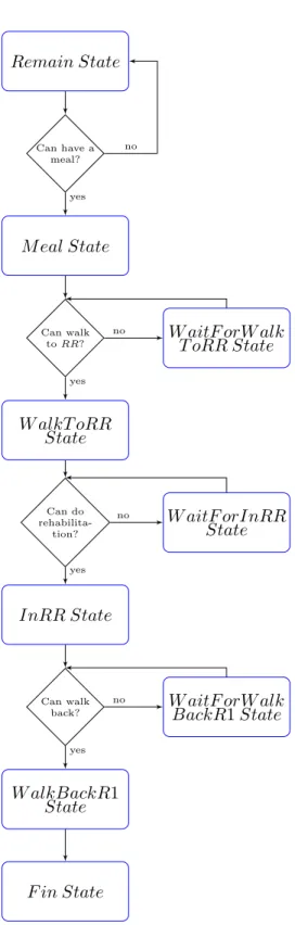
Figure 5.1 shows the state transition that represents steps of doing activities for each patient in group G1. There are 9 states, which can be separated into two groups. The first group, we call group of Doing states, consists of M eal state, W alkT oRR state, InRR state and W alkBackR1 state. The group of Doing states represents the states that refers to the main activities, that each patient needs to do. For the second group, we call group of W aiting states, consists of Remain state, W aitF orW alkT oRR state, W aitF orInRR state, W aitF orW alkBackR1 state and F in state. The group of W aiting states represents the states that each patient are waiting for doing the main activities when the resources are not sufficient to do. Each patient may or may not be in the states in the group of W aiting states, but they must be in all states of the group of Doing state.

In the initial step, each patient is in the Remain state and has a state transition as follows:

· In the Remain state : patient must change state to M eal state for having a meal. However, before changing state, it needs to check that can the patient has a meal? The condition to check is that the number of remaining nurses must suffice to help. If so, the patient must move to M eal state. Otherwise, he must wait in Remain state until the condition holds.

(32)

· In the Meal state : patient must take time to have a meal at least 30 minutes, but at most 60 minutes before changing state to W alkT oRR state. However, before changing state, it needs to check that can the patient walks? The condition to check is that the number of remaining nurses must suffice. If so, the patient must change to W alkT oRR state. Otherwise, he must wait in W aitF orW alkT oRR state until the number of nurses suffices.

· In the WaitForWalkToRR state : patient must always try to change state to W alkT oRR state. If the condition to change the state holds, the patient must change the state immediately.

· In the WalkToRR state : patient must take time to walk at least 3 minutes, but at most 5 minutes before changing state to InRR state. However, before changing state, it needs to check that can the patient do a rehabilitation? The condition to check is that there is a free space in the rehabilitation room. If so, the patient must change to InRR state. Otherwise, he must wait in W aitRR state until the condition holds.

· In the WaitForInRR state : patient must always try to change state to InRR state. If the condition to change the state holds, the patient must change the state imme-diately.

· In the InRR state : patient must take time to do a rehabilitation at least 30 minutes, but at most 45 minutes before changing state to W alkBackR1 state. However, be-fore changing state, it needs to check that can the patient walks back? The condition to check is that the number of remaining nurses must suffice. If so, the patient must change to W alkBackR1 state. Otherwise, he must wait in W aitF orW alkBackR1 state until the number of nurses suffices.

· In the WaitForWalkBackR1 state : patient must always try to change state to W alkBackR1 state. If the condition to change the state holds, the patient must change the state immediately.

· In the WalkBackR1 state : patient must take time to walk back at least 3 minutes, but at most 5 minutes before changing state to F in state.

· In the Fin state : if the patient is in the F in state, it means that the patient has already done all activities, and he must not change state anymore.

Note that when each patient changes the state, he must release all acquired resources before trying to change the state. For example, if the patient is in the M eal state and wants to change the state to W alkT oRR state, he must release the resource of one nurse to the system before changing.

For the patients in group G2, we use the same state transition to represent their steps of doing activities. However, there are some different points between the state transitions of patients in group G1 and G2, which are:

(33)

· the names of states, which represent the different activities, in state transitions; · the conditions, which are used to check that can patients change states?;

· the limitation of time that patients must take to do each activity; and

· the resource of spaces in the bath room BR that is used instead of spaces in the reha-bilitation room RR.

5.2 Specification and Solving Problem in Alloy

5.2.1 Specification in Alloy

To specify the hospital problem in Alloy, we specify the whole system with atoms and rela-tions that are represented by signatures and fields. Moreover, we describe the constraints and state transitions with facts.

Specification of Atoms and Relations of Hospital Problem

For the hospital problem, there are 3 abstract signatures, 23 signatures, and 3 fields. The signatures are:

· Patient : we specify the signatures of patients as in Program 5.1, from line 4 to line 11. The signature P atient is an abstract signature, which consists of three subsig-natures. The three subsignatures are:

· Patient1 : represents a set of atoms of patients in group G1, · Patient2 : represents a set of atoms of patients in group G2,

· NoPatient : represents an atom of a dummy patient that does not refer to any patient in the system. This atom is used to associate with nurses that are not helping any patient in each time.

· Nurse : we specify the signature of nurses as in Program 5.1, from line 13 to line 15. The signature N urse represents a set of atoms of nurses.

· Activity1 : we specify the signature of activity1 as in Program 5.1, from line 17 to line 26. The signature Activity1 represents the set of all states that refers to steps of doing activities for each patient in group G1. It is an abstract signature that consists of 9 subsignatures. Each subsignature represents each state of activity, and each one consists of only one atom.

· Activity2 : we specify the signature of activity2 as in Program 5.1, from line 28 to line 37. The signature Activity2 represents the set of all states that refers to steps of doing activities for each patient in group G2. Same as Activity1, it is an abstract signature that consists of 9 subsignatures.

(34)

Remain State Can have a meal? M eal State Can walk to RR? W alkT oRR State

W aitF orW alk T oRR State Can do rehabilita-tion? InRR State W aitF orInRR State Can walk back? W alkBackR1 State

W aitF orW alk BackR1 State F in State yes yes no yes no yes no no

(35)

· Time : we specify the signature of time as in Program 5.1, from line 1 to line 2. Since the signature T ime is defined as a parameter of module Ordering, the atoms in its set have an order. Each atom in set T ime is used to represent each minute of the system.

The fields are:

· doActivity1 : we specify the field doActivity1 in the signature P atient1. The field doActivity1 is a ternary relation that associating each atom of P atient1 with relation from Activity1 to T ime, which each atom of T ime belongs to exactly one atom of Activity1. This relation represents the activity that each patient in group G1 does in each minute. Moreover, for each minute, each patient in group G1 must do exactly one activity.

· doActivity2 : we specify the field doActivity2 in the signature P atient2. The field doActivity2 is a ternary relation that associating each atom of P atient2 with relation from Activity2 to T ime, which each atom of T ime belongs to exactly one atom of Activity2. This relation represents the activity that each patient in group G2 does in each minute. Moreover, for each minute, each patient in group G2 must do exactly one activity.

· help : we specify the field help in the signature N urse. The field help is a ternary relation that associating each atom of N urse with relation from P atient to T ime, which each atom of T ime belongs to exactly one atom of P atient. This relation rep-resents the patient that each nurse helps in each minute. Moreover, for each minute, each nurse must help exactly one patient. However, in the case of nurse that does not help any patient, the nurse must associate with the dummy patient,N oP atient, in that minute.

Note that the relations of the system are used to represent the states of system, which record that in each minute, each patient does which activity and each nurse helps which patient?

Example 5.2.1.1 . Given following sets of P atient1, N urse, and T ime: Patient1 = {(P0), (P1), (P2)}

Nurse = {(N0), (N1)} Time = {(T0), (T1), (T2)}

If in the relation doAcitivity1 consists of a tuple (P 0, M eal, T 2), it means that at the minute T 2, patient P 0 has a meal. Moreover, if in the relation help consists of a tuple (N 0, P 0, T 2), it means that at the minute T 2, Nurse N 0 helps patient P 0.

Program 5.1: Specification of signatures and fields of Hospital Problem 1 open u t i l / o r d e r i n g [ Time ]

(36)

3 4 abstract s i g P a t i e n t {} 5 s i g P a t i e n t 1 extends P a t i e n t { 6 d o A c t i v i t y 1 : A c t i v i t y 1 one −> Time 7 } 8 s i g P a t i e n t 2 extends P a t i e n t { 9 d o A c t i v i t y 2 : A c t i v i t y 2 one −> Time 10 } 11 one s i g N o P a t i e n t extends P a t i e n t {} 12 13 s i g Nurse { 14 h e l p : P a t i e n t one −> Time 15 } 16 17 abstract s i g A c t i v i t y 1 {}

18 one s i g Remain extends A c t i v i t y 1 {} 19 one s i g Meal extends A c t i v i t y 1 {}

20 one s i g WaitForWalkToRR extends A c t i v i t y 1 {} 21 one s i g WalkToRR extends A c t i v i t y 1 {}

22 one s i g WaitForInRR extends A c t i v i t y 1 {} 23 one s i g InRR extends A c t i v i t y 1 {}

24 one s i g WaitForWalkBackR1 extends A c t i v i t y 1 {} 25 one s i g WalkBackR1 extends A c t i v i t y 1 {}

26 one s i g Fin extends A c t i v i t y 1 {} 27

28 abstract s i g A c t i v i t y 2 {}

29 one s i g Remain2 extends A c t i v i t y 2 {} 30 one s i g Meal2 extends A c t i v i t y 2 {}

31 one s i g WaitForWalkToBR extends A c t i v i t y 2 {} 32 one s i g WalkToBR extends A c t i v i t y 2 {}

33 one s i g WaitForInBR extends A c t i v i t y 2 {} 34 one s i g InBR extends A c t i v i t y 2 {}

35 one s i g WaitForWalkBackR2 extends A c t i v i t y 2 {} 36 one s i g WalkBackR2 extends A c t i v i t y 2 {}

37 one s i g Fin2 extends A c t i v i t y 2 {} Specification of State Transitions

The state of Alloy is recorded as a tuple in the relations. We use f act to define state transitions as the constraints that are assumed always to hold. Moreover, we use predicate to define operators that are used to assign the values of variables in the state when changing minutes of time. As we described in the section 5.1, the state transitions that represent step of doing activities of patients in group G1 and G2 are the same (just the

(37)

names and some conditions are difference). So, we’ll refer just to the specification of state transitions of each patient in group G1.

Program 5.2 represents the specification of state transitions of hospital problem in Alloy. We use predicate as operators to assign the values of variables in the states (values of atoms in the tuples in each relation). In this system, there are two roles of predicate.

The roles of predicate are:

· Assigning the initial state to all patients : we specify the predicate that is used to assign the values of initial state as in Program 5.2, from line 1 to line 4.

The predicate is named init, and it has one parameter. The parameter is a given minute of time t, that is set to be an initial minute of the system. In the predicate, it assigns the tuples, which associate each patient in group G1 with a relation from atom Remain to a given minute t (and each patient in group G2 with a relation from atom Remain2 to a given minute t), to the relation doActivity1 (and doActivity2). It represents that in the initial state of the system, all patients must be in the Remain state.

· Assigning the state to a given patient and minute : in the system, there are 9 predicate paragraphs of this type of predicate for each group of patients (18 predicate paragraphs for two groups of patients). Each one is used to assign each state of doing activity to a given patient at a given minute. Since all 18 predicates are the same (just changes the names of predicates and names of states), we’ll show only one predicate paragraph that is specified as in Program 5.2, from line 6 to line 8.

The predicate is named haveM eal, and has two parameters. The parameters are a given minute of time t0, and a given patient p in group G1. In the predicate, it assigns the tuple, which associate the patient p with a relation from atom M eal to a given time t0, to the relation doActivity1. It represents that at the given time t0, the given patient p must be in the M eal state.

Moreover, we use f act, is named T races, to define state transitions as in Program 5.2, from line 10 to line 31.

At first, in line 11, we call the predicate init to assign the initial state by parsing the return value of operator f irst as a parameter. The operator f irst returns the first atom of order in the set T ime. And then, we define the constraint for state transition, as from line 12 to 30, that for each minute t, each patient p in group G1 must be assigned the next state of activity in the next minute t0, which depends on the current state (where t represent a current minute and t0 represents a next minute that follows t from the order in set T ime). To check the current states of activities of each patient in group G1, we check the tuples in the relation doActivity1 by using dot join operator. Moreover, to assign the next states of activities of each patient in group G1, we use the predicate that are described above, by parsing the next time t0 and each patient p as parameters.

We assign the next states of activities for each patient in state transition depends on the current states. There are 9 cases of the current states as following:

(38)

· Remain state (p.doActivity1.t = Remain) : the next state can be M eal state, or the same state (Remain state).

· Meal state (p.doActivity1.t = Meal) : the next state can be W aitF orW alkT oRR state, W alkT oRR state, or the same state (M eal state).

· WaitForWalkToRR state (p.doActivity1.t = WaitForWalkToRR) : the next state can be W alkT oRR state, or the same state (W aitF orW alkT oRR state). · WalkToRR state (p.doActivity1.t = WalkToRR) : the next state can be InRR

state, W aitF orInRR state, or the same state (W alkT oRR state).

· WaitForInRR state (p.doActivity1.t = WaitForInRR) : the next state can be InRR state, or the same state (W aitF orInRR state).

· InRR state (p.doActivity1.t = InRR) : the next state can be W aitF orW alkBackR1 state, W alkBackR1 state, or the same state (InRR state).

· WaitForWalkBackR1 state (p.doActivity1.t = WaitForWalkBackR1) : the next state can be W alkBackR1 state, or the same state (W aitF orW alkBackR1 state). · WalkBackR1 state (p.doActivity1.t = WalkBackR1) : the next state can be F in

state, or the same state (W alkBackR1 state).

· Fin state (p.doActivity1.t = Fin) : the next state can be only F in state (it will not change the state anymore).

Program 5.2: Some Parts of Specification of State Transitions in Alloy 1 p r e d i n i t ( t : Time ) { 2 a l l p : P a t i e n t 1 | p . d o A c t i v i t y 1 . t = Remain 3 a l l q : P a t i e n t 2 | q . d o A c t i v i t y 2 . t = Remain2 4 } 5 6 p r e d haveMeal ( t ’ : Time , p : P a t i e n t 1 ) { 7 p . d o A c t i v i t y 1 . t ’ = Meal 8 } 9 10 f a c t T r a c e s { 11 f i r s t . i n i t 12 a l l t : Time − l a s t | l e t t ’ = t . n e xt | 13 a l l p : P a t i e n t 1 | 14 p . d o A c t i v i t y 1 . t = Remain i m p l i e s 15 ( haveMeal [ t ’ , p ] o r notDo [ t ’ , p ] ) 16 e l s e p . d o A c t i v i t y 1 . t = Meal i m p l i e s

17 ( walkRR [ t ’ , p ] o r waitForWalkRR [ t ’ , p ] o r haveMeal [ t ’ , p ] ) 18 e l s e p . d o A c t i v i t y 1 . t = WaitForWalkToRR i m p l i e s

JAIST Repository: A survey of Alloy specification language and comparison with an algebraic specification language [課題研究報告書]