DRAWING BERS EMBEDDINGS OF THE TEICHMULLER SPACE OF ONCE PUNCTURED TORI (Hyperbolic Spaces and Related Topics II)

(1)

DRAWING BERS EMBEDDINGS OF THE

TEICHM\"ULLER

SPACE OF

ONCE PUNCTURED TORI

大阪市立大学理学部小森洋平 (Yohei Komori)

匠都大学理学部須川敏幸 (Toshiyuki Sugawa)

奈良町子大学理学部和田昌昭 (Masaaki Wada)

奈良女子大学理学部山下靖 (Yasushi Yamashita)

1. INTRODUCTION Let $\Gamma$be

a

Fuchsiangroupacting

on

the unit disk$\mathrm{D}$uniformizing

a

once

punctured torus

$S$ and $B_{2}(\mathrm{D}, \Gamma)$ the complexBanach space of holomorphic quadratic differentials for $\Gamma$

on

$\mathrm{D}$ withbounded norm.

It is well known that the complexdimension of$B_{2}(\mathrm{D}, \Gamma)$ is

one

and

we can

embed the Teichm\"uller space $T(\Gamma)$ of $\Gamma$ in

$B_{2}(\mathrm{D}, \Gamma)$ by the Bers projection $\Phi$

as a

bounded contractible open subset.

In 1972, Bers wrote ([Bers 1972]

page

278)

Unfortunately, there is

no

known method to decide whether

a

given$\phi\in B_{2}(L, G)$

belongs to $T(G)$

.

This is

so even

if_{$d=\dim B_{2}(L, G)<\infty$}

.

_{Even the}

case

_$d=1$

is untractable.

($G$ is a Fuchsian group acting on the upper halfplane and _$L$ is the lower half_plane.)

In this paper

we

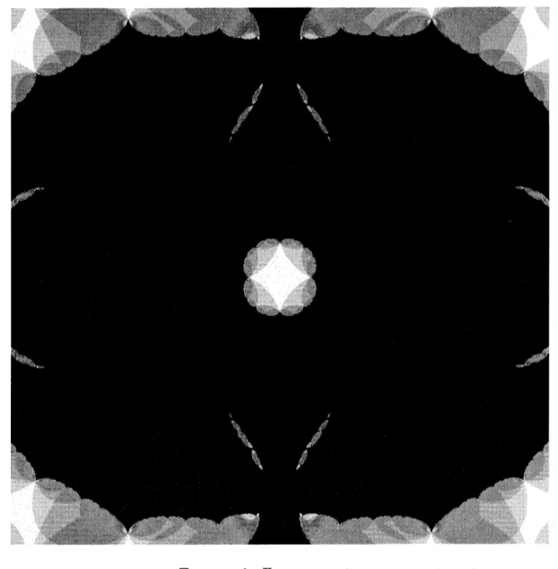
show the pictures of $\Phi(T(\Gamma))$ in $B_{2}(\mathrm{D}, \Gamma)$ for several $\Gamma$ and explain

our

algorithm to produce such pictures. See Figure 1 for example. _{We claim that the}

component located at the center ofthe picture is equal to $\Phi(T(\Gamma))$

.

To describethe ideaof the algorithm,let

us

recall

some

basicfacts inTeichm\"ullertheory.

([Shiga 1987])

For every $\phi$ in $B_{2}(\mathrm{D}, \Gamma)$, there exists

a

locally univalent meromorphic function $f_{\phi}$

on

$\mathrm{D}$ with $\{f_{\phi}, z\}=\phi(z)$ where $\{f, \cdot\}$ is the Schwarzian derivative of _$f$

.

After certain normal-ization (see section 2), $f_{\phi}$ is uniquely determinedby $\phi$and induces

a

grouphomomorphism

$\theta_{\phi}$ : $\Gammaarrow \mathrm{P}\mathrm{S}\mathrm{L}(2, \mathbb{C})$ defined by

$f_{\phi}\mathrm{o}\gamma=\theta_{\phi}(\gamma)\mathrm{o}f_{\phi}$, $\gamma\in\Gamma$

.

We call $\theta_{\phi}$ the holonomy representation of $\Gamma$ associated with

$\phi\in B_{2}(\mathrm{D}, \Gamma)$

.

We consider the set $K(\Gamma)$ of$\phi$ in $B_{2}(\mathrm{D}, \Gamma)$ such that $\theta_{\phi}(\Gamma)$ is

a

Kleinian group. Then

Theorem 1.1 ([Shiga 1987]). $\Phi(T(\Gamma))$ is equal to the component

of

Int$K(\Gamma)$ containing

the origin.

Therefore

we

will draw the pictures of$K(\Gamma)$ in $B_{2}(\mathrm{D}, \Gamma)$ for given $\Gamma$ and that the algo-rithm involves the following two steps: for each element $\phi$ in $B_{2}(\mathrm{D}, \Gamma)\cong \mathbb{C}$,

we

Step 1: compute the holonomy representation $\theta_{\phi}$ and

Step 2: decide whether the image $\theta_{\phi}(\Gamma)$ in $\mathrm{P}\mathrm{S}\mathrm{L}(2, \mathbb{C})$ is discrete. Each step will be discussedin section 2 and 3.

(2)

2. HOLONOMY REPRESENTATION

In this section

we

will describe

an

algorithm which

t.akes

as

input

an

element $\phi$ of

$B_{2}(\mathrm{D}, \Gamma)$ and returns

a

holonomy representation $\theta_{\phi}$

.

2.1. Monodromy homomorphism. Let $\phi\in B_{2}(\mathrm{D}, \Gamma)$

.

We associate with $\phi$ the

mero-morphic function $f_{\phi}=\eta_{1}/_{l}\eta_{0}$, where $\eta_{1}$ and $\eta_{2}$

are

linearly independent solutions of the

differential equation

(1) $2\eta^{l/}+\emptyset\eta=0$,

normalized by the initial conditions

$\eta_{0}(0)=1$ $\eta_{0}’(0)=^{\mathrm{o}}$

$\eta_{1}(0)=0$ $\eta_{1}’(0)=1$

.

Then $\{f_{\phi}, z\}=\phi(z)$

on

$\mathrm{D}$

as

expected.

To illustrate how

we

get the holonomy representation, let

us

consider the solutions of

(1). In view of $\Gamma$-invariance of $\phi(z)dz^{2}$,

we see

that if $\eta$ is a solution of (1), then

so

is

$\gamma^{*}\eta:=(\eta 0\gamma)(\gamma)^{-}/1/2$ for every $\gamma\in\Gamma$

.

In particular, since $(\eta_{0}, \eta_{1})$ is

a

basis of solutions of

(1),

we can

write

$\gamma^{*}\eta_{0}=D\eta 0+C\eta 1$, . $\gamma^{*}\eta_{1}=B\eta 0+A\eta 1$,

for

some

complex numbers $A,$$B,$$C$ and $D$

.

By setting

$\theta_{\phi}(\gamma)=$ ,

we

have

$f_{\phi^{\mathrm{O}}} \gamma=\frac{\gamma^{*}\eta_{1}}{\gamma\eta_{0}}*=\frac{B\eta_{0}+A\eta_{1}}{D\eta_{0}+c_{\eta 1}}=\frac{Af+B}{Cf+D}=\theta\phi(\gamma)\mathrm{o}f_{\emptyset}$

for each $\gamma$ and this is the desired homomorphism associated with

$\phi$

.

So

our

task is to

compute suchcomplexnumbers $A,$$B,$$C$ and$D$ for each generator ofgroup F. But to make

our

calculation easier,

we

will work with

a

4-times punctured sphere.

2.2. Commensurabilityrelations. Let $\Gamma$be

a

Fuchsiangroupuniformizing

a once

punc-tured torus $T$ and $(\alpha, \beta)$

a

standardgeneratorpairof$\Gamma$, i.e. $\alpha$ and$\beta$ freelygenerate $\Gamma$, both

are

hyperbolic, the commutator $[\alpha, \beta]$ is parabolic and the intersection number $\alpha\cdot\beta=1$

.

Then $T$ admits an intermediate covering space which is the plane

$\mathbb{C}$ punctured at a lattice

$L_{\tau}=\{m+n\tau;m, n\in \mathbb{Z}\}$ so that $\alpha$ and $\beta$ correspond to the generators

$zarrow z+1$, $zarrow z+\tau$

for $L_{\tau}$

.

We may

assume

that $s\tau\infty>0$

.

Now consider the 4-times punctured sphere $S$ and the $(2, 2, 2, \infty)$-orbifold $\mathcal{O}$ (i.e., the

orbifold withunderlying space

a

punctured sphere and with three

cone

points of

cone

angle

$\pi)$ which have $\mathbb{C}-L_{\tau}$

as

the

common

covering space. More precisely, let $G_{S}$ and

$G_{\mathcal{O}}$ be

the

groups

of transformations

on

$\mathbb{C}-L_{\mathcal{T}}$ generated by $\pi$-rotations about points in $L_{\tau}$ and

$\frac{1}{(2}L_{\mathcal{T}}:=\{\mathrm{a}\mathrm{n}\mathrm{d}T=((m+n\tau_{L_{\mathcal{T}}})\mathbb{C}-/2\cdot,m, n\in \mathbb{Z}\}\mathrm{r}_{\mathrm{h}\mathrm{t}}\mathrm{e}\mathrm{S}\mathrm{p}\mathrm{e}\mathrm{C}\mathrm{t}\mathrm{i}_{\mathrm{V}\mathrm{e}1}\mathrm{y}.\mathrm{T})/L_{\mathcal{T}})$

.

$\mathrm{N}_{0}\mathrm{t}\mathrm{e}\mathrm{t}\mathrm{a}\mathrm{W}\mathrm{e}\mathrm{h}\mathrm{a}\mathrm{v}\mathrm{e}\mathrm{f}\mathrm{i}\mathrm{n}\mathrm{i}\mathrm{t}\mathrm{e}\mathrm{c}\mathrm{o}\mathrm{V}\mathrm{e}\mathrm{r}(\mathrm{h}\mathrm{e}\mathrm{n}S=\mathbb{C}-L)\mathrm{i}\mathrm{n}\mathrm{g}\mathrm{S}\tau^{\tau}arrow \mathcal{O}\mathrm{a}\mathrm{n}\mathrm{d}Sarrow/Gs\mathrm{a}\mathrm{n}\mathrm{d}\mathcal{O}=(\mathcal{O}\mathbb{C}.-L_{\mathcal{T}})/G_{o}$

Let $\Gamma_{S}$ and $\Gamma_{\mathcal{O}}$ be the covering group of the universal

cover

$\mathrm{D}arrow(\mathbb{C}-L)_{\tau}arrow S$ and

$\mathrm{D}arrow(\mathbb{C}-L_{\mathcal{T}})arrow \mathcal{O}$ respeotively. Since $L_{\tau}\triangleleft G_{\mathcal{O}}$ and

(3)

$\Gamma_{S}\triangleleft\Gamma_{\mathcal{O}}$

.

In particular, _{$B_{2}(\mathrm{D}, \Gamma_{\mathcal{O}})\subset B_{2}(\mathrm{D}, \Gamma)$} and _{$B_{2}(\mathrm{D}, \mathrm{r}_{o})\subset B_{2}(\mathrm{D}, \Gamma_{S})$}

.

Since these

are

all 1-dimensional vector spaces, all three are equal and we conclude that $B_{2}(\mathrm{D}, \Gamma S)=$ $B_{2}(\mathrm{D}, \Gamma)$

.

Recall that

we can use a

single global coordinate $z$

on

$S$: $S=\hat{\mathbb{C}}-\{\mathrm{o}, 1, \infty, \lambda\}$

.

Without loss of generality

we

may

assume

that the lattice points $0,1,1+\tau,$$\tau$

on

$L_{\tau}\subset \mathbb{C}$

correspond to the punctures $0,1,$$\infty,$$\lambda$ of $S$

.

Let

$p$ : $\mathrm{D}arrow S\cong\hat{\mathbb{C}}-\{0,1, \infty, \lambda\}$ be the

projection and $B_{2}(S)$ the Banach space of bounded holomorphic quadratic differentials

on

$S$

.

By definition, the spaces $B_{2}(\mathrm{D}, \mathrm{r}_{S})$ and $B_{2}(S)$

are

isomorphic via the pull-back

$p_{2}^{*}$ : $B_{2}(S)arrow B_{2}(\mathrm{D},$$\Gamma_{s)}$ defined by$p_{2}^{*}\psi=\psi \mathrm{o}p\cdot(p’)^{2}$

.

In particular, dimension of_{$B_{2}(S)$} is

equal to

one.

Since the rational function

(2) $\psi \mathrm{o}(Z)=\frac{1}{z(z-1)(\chi-\lambda)}$

belongs to $B_{2}(S),$ $\psi_{0}$ forms

a

basis of the vector space _{$B_{2}(S)$}

.

Therefore each element

$\phi\in B_{2}(\mathrm{D}, \Gamma)=B_{2}(\mathrm{D},$ $\Gamma_{s)}$

can

be written

as

$\phi=t\phi_{0}$ where $t$ is

a

complex number and

$\phi_{0=}p^{*}2(\psi 0)$

.

2.3. The monodromy ofa4-times punctured sphere. Now for each$\phi=t\phi_{0}$, consider

the developing map $f_{\phi}$ :

$\mathrm{D}arrow\hat{\mathbb{C}}$

.

Our idea is to compute $f_{\phi}$

on

$S$ instead ofD.

So

we

change the independent variable of $f_{\phi}(x)$ by function $x=p^{-1}(z)$ locally

near

$\mathrm{O}\in \mathrm{D}$ and refer to the independent variable

$z$ on $\hat{\mathbb{C}}-\{0,1, \infty, \lambda\}$

near

$p(\mathrm{O})$

.

Set $P=p^{-1}$

and $g(z):=f\phi(P(z))$

.

Then

we

have

(3) $\{g, z\}=\{f_{\phi}, P(z)\}(P’(z))^{2}+\{P, z\}=t\psi_{0}(Z)+\{P, z\}$

.

and to find $g$ (or $f_{\phi}$ as a functionof $z$)

we

must consider the corresponding linear second order equation

(4) $2y^{ll}+\{_{\mathit{9}}, z\}y=0$

and express $g$

as

the ratio of two independent solutions of this equation. For $\{P, z\}$

we use

the next lemma:

Lemma 2.1 ([Hempel 1988], [Kra 1989]). $\{P, z\}$ is

of

the

form

(5) $\{P, z\}=\frac{1}{2z^{2}}+\frac{(1-\lambda)^{2}}{2(z-1)^{2}(z-\lambda)2}+\frac{c(\lambda)}{z(z-1)(Z-\lambda)}$

.

on $S$ where $c(\lambda)$ is a constant determined by $\lambda$ and called accessory parameter.

By the above lemma and (3), $\{g, z\}$ is globally defined

on

$\hat{\mathbb{C}}-\{0,1, \infty, \lambda\}$

.

Combining

(2),(3) and (5), the equation (4) to solveis

(4)

Now

we

describe the computation of the monodromy. Let $\gamma_{S}$ be

an

element of $\Gamma_{S}$ We start with

an

pair $(y_{0}, y_{1})$ of independent solutions of (6) from

a

certain point $z_{0}$

on

$S$

normalized by the initial conditions

$y_{0}(Z\mathrm{o})=1$ $y_{0}^{l}(z_{0})=0$

$y_{1}(z_{0})=0$ $y_{1}^{l}(z\mathrm{o})=1$

.

Then

we

continue them analyticallyalong

a

closed path of$S$ corresponding to $\gamma_{S}$

.

Return-ing to the startReturn-ing point,

we

will arrive with

a new

pair of solutions $(\mathrm{Y}_{0}, \mathrm{Y}_{1})$

.

However, these

new

solutions must be linear combinations ofthe original solutions. Thus

we

have

$\mathrm{Y}_{0}=Dy_{0}+Cy_{1}$, $\mathrm{Y}_{1}=By_{0}+Ay_{1}$,

for

some

complex numbers $A,$ $B,$$C$ and $D$

.

We define

$\theta_{\psi}(\gamma S)=$

for each$\gamma s\in\Gamma_{S}$

.

Let

us

compare $g(=f_{\phi}(p^{-1})$ and $h:=y_{1}/y_{0}$

.

Though both $g$ and $h$ satisfy the

same

equation (6), the initial conditions at $z_{0}$

are

not the

same.

This difference leads to a

conjugationfrom

one

of$\theta_{\phi}(\Gamma s)$

or

$\theta_{\psi}(\Gamma_{S})$ to the other. Therefore

we

have shown that

Lemma 2.2. The monodromies $\theta_{\phi}$ and $\theta_{\psi}$ are essentially the same. (Up to conjugacy)

So

we can

do

our

calculations

on

$S$ using (6).

2.4. Punctured torus groups. Now it

seems

like it’s time to compute $\theta_{\psi)}(\alpha)$ and $\theta_{\vee)}(\alpha)$

by solving (6) along the corresponding paths in $S=\hat{\mathbb{C}}-\{0,1, \infty, \lambda\}$

.

Unfortunately, though $\alpha$ and$\beta$

are

in $\Gamma$, they

are

not in $\Gamma_{S}$ for which

we

have $\theta_{\psi}$

.

In other words, $\alpha$ and $\beta$ do not correspond to the closed paths in $S$

.

So

we

need

a

little

more

calculation to end this section.

First, observe that$\iota \mathrm{r}[\theta_{\phi(\alpha),\theta(}\emptyset\beta)]=-2$

.

Set $x=\mathrm{t}\mathrm{r}\theta_{\phi}(\alpha),$ $y=\mathrm{t}\mathrm{r}\theta_{\phi}(\beta)$ and$z=\mathrm{t}\mathrm{r}\theta_{\phi(\alpha}$

.

$\beta)$

.

From the trace identity $2+\mathrm{t}\mathrm{r}[X, \mathrm{Y}]=(\mathrm{t}\mathrm{r}X)^{2}+(\mathrm{t}\mathrm{r}\mathrm{Y})^{2}+(\mathrm{t}\mathrm{r}X\mathrm{Y})^{2}-\mathrm{t}\mathrm{r}X$tr$\mathrm{Y}$tr$X\mathrm{Y}$,

we

obtain:

(7) $x^{2}+y^{2}+Z=X2yz$

.

Conversely, given any triple $(x, y, z)$ satisfying (7),

we

can

reconstruct the image of the

group $\Gamma$ up to conjugacy. We call suchtriple of complex numbers Markov triple.

Thus itsuffices tocompute $x$ and$y$

.

Again bytrace identitytr$A$tr$B=\mathrm{t}\mathrm{r}AB+\mathrm{t}\mathrm{r}AB^{-1}$ $y=\sqrt{-\mathrm{t}\mathrm{r}\theta_{\psi}(\beta^{2})+2}$

.

Now

we can

calculate $\theta_{\psi}(\alpha^{2})$ and$\theta_{\psi}(\beta^{2})$ usingequation (6) because $\alpha^{2}$ and$\beta^{2}$

are

in$\Gamma_{s}$ The closed loop in $S$ separating $\{0,1\}$ and $\{\infty, \lambda\}$ corresponds to $\alpha^{2}$ and the

one

separating

(5)

3. $\mathrm{J}_{\mathrm{o}\mathrm{R}\mathrm{G}\mathrm{E}\mathrm{N}\mathrm{s}\mathrm{E}}\mathrm{N}’ \mathrm{S}$ THEORY TO DECIDE DISCRETENESS

The input ofthe algorithmofthis section is

a

Markovtriple andthe output is the

answer

“discrete”

or

“indiscrete”.

The general idea is to try to construct the Ford fundamental region of the given Markov

triple though it may not have

a

discrete group image in $\mathrm{P}\mathrm{S}\mathrm{L}(2, \mathbb{C})$

.

In this

case

the

$\mathrm{t}\mathrm{e}\mathrm{r}\mathrm{m}$“$\mathrm{F}_{0}\mathrm{r}\mathrm{d}$ fundamental region” does not make

sense

and

our

process of constructing it

will fail. Then

we

will search for the evidence of its indiscreteness.

We have two remarks. First, this algorithm is based

on

the Jorgensen’s theory

on once

punctured tori [Jorgensen]. The exposition ofthis theory with proofs and a generalization

is in preparation in [Akiyoshi et al.]. Next, this algorithmmay not halt in a finite time for

some

inputs. The

cases

where $\mathbb{H}^{3}/\theta_{()}x,y,z(\Gamma)$ is

a

punctured torus bundle

or

geometrically

infinite

are

the examples. In practice,

we

will stop

our

calculation at

a

certain time and

answer

“undecided”.

3.1. Conditions for discreteness. Before describing

our

procedure, let

us

recall the

well known conditions for discreteness for the group action. The first one is Poincar\’e’s

fundamental polyhedron theorem and the next one is due to Shimezu and Leutbecher.

Theorem 3.1. Let $\Psi$ be a proper isometric side pairing

for

an convex polyhedron _$P$ in

$\mathbb{H}^{3}$

such that the hyperbolic

_manifold

$M$ obtained by gluing together the sides

of

$P$ by $\Psi$ is

complete. Then the group $\Gamma$ generated by $\Psi$ is discrete.

Lemma 3.2. Suppose that a discrete subgroup $\Gamma$

of

$\mathrm{S}\mathrm{L}(2, \mathbb{C})$ contains

any $\in\Gamma$, we have $|c|\geq 1$

if

$c\neq 0$

.

We will

use

the theorem3.1 to show that a group is discrete and lemma 3.2 to show that

a

group is indiscrete.

3.2. Isometric hemispheres. Let $(x, y, z)$ be

a

Markov triple. We

can

reconstruct $\theta$ up

to conjugacy using Jorgensen’s normalization [Jorgensen]:

(8) $\theta(\alpha)=\frac{1}{x}$ , $\theta(\beta)=\frac{1}{x}$

.

Note that

(9) $\theta(\alpha\beta)=(_{X}^{X}$ $-1/x0)$ ,

$\theta(K)--$

where $K=[\alpha, \beta]$

.

The isometric hemispheres of$\alpha,$ $\alpha\beta$ and $\beta$

are

centered at $-\chi/xy,$ $0$ and $y/zx$ with radii

$1/y,$ $1/x$ and $1/z$ respectively. The isometric hemispheres of$\alpha^{-1},$ $(\alpha\beta)^{-1}$ and $\beta^{-1}K^{-1}$

are

the translated images of the above three hemispheres by $z\vdasharrow z+1$

.

Since $\theta(\Gamma)$ contains

the action $\theta(K)$ of translation $z\vdasharrow z+2$,

we

have

an

$\mathrm{b}\mathrm{i}$-infinite sequence of translated

(6)

denote these isometric hemispheres $I(\gamma)$ of$\gamma\in\Gamma$ in this sequence by

(10)

. .

.

,$I_{-4}=I(\alpha^{-1}K),$$I-3=I((\alpha\beta)-1K),$$I_{-2}=I(\beta^{-1}),$ $I-\iota=I(\alpha),$$I_{0}=I(\alpha\beta)$,

$I_{1}=I(\beta),$$I_{2}=I(\alpha^{-1}),$ $I_{3}=I((\alpha\beta)^{-}1),$$I_{4}=I(\beta-1K-1),$$I5=I(\alpha K^{-1}),$$\ldots$

Note that $I_{n}+1=I_{n+3}$ for any $n\in$ Z. Set $I_{(x.y,z)}:=\{I_{n}\}$

.

We will try to find the

set of Markov triples $\Sigma=\{(x, y, z), (xyz^{\dagger})/,/,, \ldots\}$ such that the isometric hemispheres

$I_{(x,y.z)}.’ I’(x,.y’,\mathcal{Z}’),$$\ldots$ formthe boundaryof the Fordfundamentalregion. We begin by putting $\Sigma=\{(x, y, z)\}$ and check

some

conditions for this $\Sigma$ whose output is

one

of:

Case 1:

we

have succeededin constructing the Ford fundamental region

so

itis discrete. Case 2: we have found that it is indiscrete,

Case 3:

we

need

more

isometric hemispheres to get the conclusion.

Observe that, if $(x, y, z)$ is

a

Markov triple, then three kinds of adjacent triples $(yz-$

$x,$ $z,$$y),$ ($z$,zx–y, $x$) and ($y,$$x$,xy–z)

are

also Markov triples which give rise to different families of infinite isometric hemispheres. The output of case 3 tells

us

which adjacent

triple is needed to (try to) construct the Ford fundamental region. After adding isometric

hemispheres ofthe chosen adjacent tripleto $\Sigma$,

we

checkthe above (but notyet mentioned)

conditions again. We continue this process until

we

reach the

cases

1 or 2.

Beforestartingthe above mainroutine,

we

mayhave to replacetheisometrichemispheres

$I_{(x,y,z)}$ by its neighbors. So

we

first explain this process in 3.3 and then describe the main

process which returns

case

1, 2or 3 in3.4. Inthe following

we

denote $(x, y, z)$ by $(x_{0}, x_{2}, X_{1})$

and the indices of$x_{i}$ should be understood modulo three. Then the radius of $I_{n}$ is $1/|x_{n}|$

.

3.3. The initial process.

3.3.1. For

a

Markov triple $(x_{0}, x_{1}, X_{2})$, if $|x_{i}|$ is less than

one

for

some

$i\in\{0,1,2\}$, the

group is indiscrete. This can be easily

seen

from Lemma 3.2 and (8). Therefore if this

happens in this process or in the main routine below,

we

will stop our calculation and say

(case 2). Otherwise go to 3.3.2.

3.3.2. First, to be

a

part of the boundary ofthe Ford region, we ask $I_{n}\cap I_{n+1}\neq \mathrm{f}\mathrm{o}\mathrm{r}$ every

$n\in \mathbb{Z}$ This is equivalent to the condition:

(11) $\exists$ triangle with edge lengths $|x_{0}|,$ $|x_{1}|$ and $|x_{2}|$

.

If this is not satisfied,

one

of$x_{i}$, say$x_{0}$, must be too big. Thus

we

replace $(x_{0}, x_{1}, X_{2})$ bythe

adjacent triplenot containing$x_{0}$ which is $(x_{1^{X}2^{-}}X_{0}, X_{2,1}x)$

.

Thus $\Sigma=\{(x_{1}x_{2}-x_{0,2,1}xX)\}$

and go back to 3.3.1. Otherwise go to 3.3.3.

3.3.3. Next, we also want that each $I_{n}$ does not covered by $I_{n-1}\cup I_{n+1}$

.

For $i\in\{0,1,2\}$,

if

(12) $|x_{i}|>|x_{i+1}+x_{i+2}I|$ and $|x_{i}|>|x_{i+1}-x_{i2}+I|$,

then this condition is not satisfied and

we

replace the triple by the adjacent triple which does not contain $x_{i}$

.

If$i=0,$ $\Sigma=\{(x_{1}X2-X0, X2, X1)\}$ and go to 3.3.1.

If

we

find

a

triple which satisfies both conditions,

we

go to 3.4.

(7)

3.4.1. Forany $\gamma$ with $I(\gamma)\in I_{(x,y,z)}$ and $(x, y, z)\in\Sigma$, let $V(\gamma)$ be the visible part of$I(\gamma)$

.

If

our

configuration given by $\Sigma$ forms the Ford region, $\theta(\gamma)(V(\gamma))$ must be equal to $V(\gamma^{-1})$

.

Besides, the action of$\theta(\gamma)$ is

1. $\pi$ rotation around the axis

on

$I(\gamma)$ connecting (center of$I(\gamma)\pm I/x_{i}$) followed by

2. the translation $zrightarrow z\pm 1$

.

The index$i$ of

$x_{i}$ and the signofthe translation above depends

on

$\gamma$

.

Since

our

configuration has

a

symmetry of translation by one, This

means

that $V(\gamma)$ must be symmetric by the

action ofthe above $\pi$ rotation.

We claim that

Proposition 3.3. This is also the $suffi_{Ci}e.nt$ condition

for

the isometric hemispheres to

form

the Ford

_fundamental

region.

The idea ofthe proof is to

use

the theorem 3.1. Since each face is symmetric, the face pairing is well defined. The properness of the face pairing

comes

from the “chain rule” of the isometric hemispheres. The completeness of the face pairing is easy.

In this

case

the

answer

is “discrete” and the result is (case 1). Otherwise goto 3.4.2.

3.4.2. To make

our

description of

our

algorithm simpler, suppose that any line segment $|I_{n},$$i_{n+1}|$ where $|I_{n},$$i_{n+1}|$ is the segment connecting the centers of $I_{n}$ and _{$i_{n+1}$}, does not

intersect with $|I_{n+2},$$in+3|$ for any $n$

.

Hence, if

we

look at the ideal boundary $\mathbb{C}$ of $\mathbb{H}^{3}$ from

$\infty$, the ideal boundary is separated into two regions by the infinite graph with vertices

$\{I_{r\iota}\}$ and edges $\{|I_{n}, i_{n+1}|\}$

.

Suppose that $V(n)$ is not symmetric for

some

$n$

.

We only consider the

cases

where $I_{n}$

intersects with $I_{n-2}$ or $I_{n+2}$, say $I_{n+2}$

.

Otherwise we stop trying to construct the Ford

region and goto 3.4.3.

Thus

we

add the adjacent Markov triple with sequence $I_{n},$ $I_{n+2}$ and something which $\mathrm{i}\mathrm{s},,(.X_{n}+2Xnx_{n+}2-x_{n+1}, x_{n})\Sigma’$

.

The output is

“$(\mathrm{c}\mathrm{a}\mathrm{s}\mathrm{e}3)$ and add $(X_{n+2}, XnXn+2-x_{n+1}, x_{n})$ to

3.4.3. Now

we

search for

a

Markov triple $(x_{0}, x_{1}, X_{2})$ with $|x_{i}|$ is less than

one

for

some

$i\in\{0,1,2\}$ to show that the group is indiscrete. We denote this condition by $(*)$

.

We start with

a

Markov triple a $\in\Sigma$

.

If $\sigma$ satisfies $(*)$,

we

finish saying (case 2). If

not, consider Markov triples adjacent to $\sigma$ in the

sense

mentioned above and check $(*)$

.

If

these three Markov triples do not satisfy $(*)$,

we

next consider the Markov triples which is

adjacent to the above three. We continue this process until

we

find the

one

whichsatisfies

$(*)$

.

In this

case we

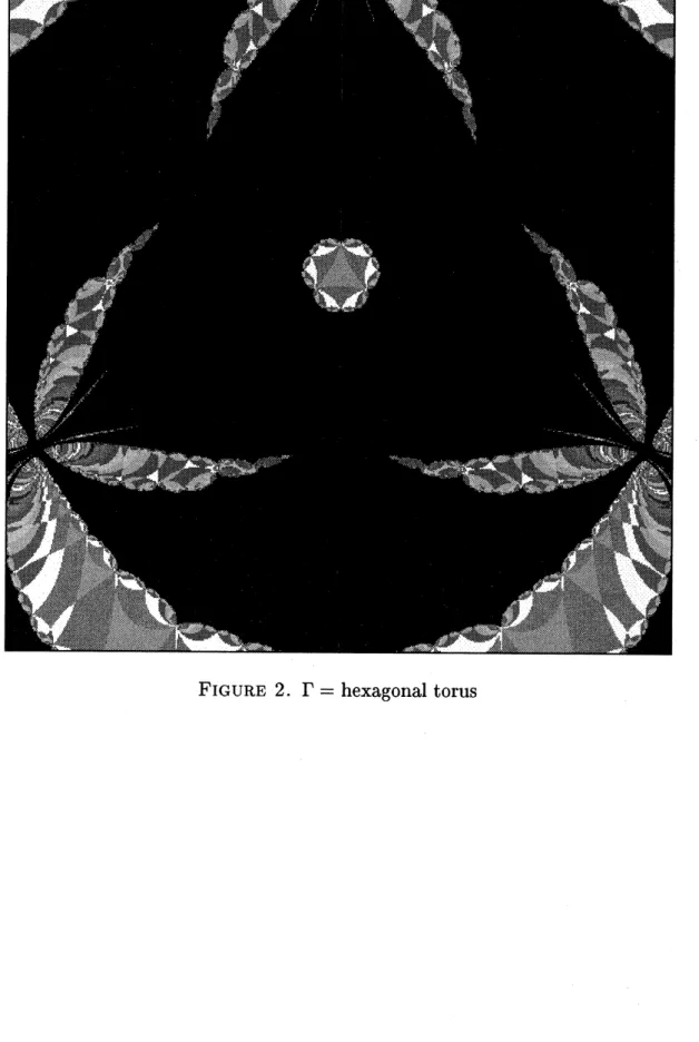
say (case 2).

4. PICTURES

We present two pictures produced by

our

method in the following pages.

5. ELECTRONIC AVAILABILITY

Files containing the program and pictures

can

be obtained from

http:$//\mathrm{v}\mathrm{i}\mathrm{v}\mathrm{a}\mathrm{l}\mathrm{d}\mathrm{i}.\mathrm{i}\mathrm{C}\mathrm{s}$

.

nara-wu.$\mathrm{a}\mathrm{C}.\mathrm{j}_{\mathrm{P}}/\sim_{\mathrm{y}\mathrm{a}\mathrm{m}\mathrm{a}\mathrm{s}\mathrm{c}}\mathrm{i}\mathrm{t}\mathrm{a}/\mathrm{S}\mathrm{l}\mathrm{i}\mathrm{e}/$

(8)

FIGURE 1. $\Gamma=\mathrm{s}\mathrm{q}\mathrm{u}\mathrm{a}\mathrm{r}\mathrm{e}$torus

REFERENCES

[Akiyoshi et al.] H. Akiyoshi, M. Sakuma, M. Wada and Y. Yamashita, Ford domains of punctured torus

groups and two-bridge knot groups, In preparation.

[Bers 1972] L. Bers, Uniformization, moduli and Kleinian groups, Bull. London Math. Soc. 4 (1972), 257-300.

[Jorgensen] T. Jorgensen, On pairs of punctured tori, Unpublished manuscript.

[Hempel 1988] J. A. Hempel, On the uniformization of the $n$-punctured sphere, Bull. London Math. Soc.

20 (1988), 97-115.

[Kra 1989] I. Kra, Accessory parameters for punctured spheres, Trans. Amer. Math. Soc. 313:2 (1989),

589-617.

[Shiga 1987] H. Shiga, Projective structures on Riemann surfaces and Kleinian groups, J. Math. Kyoto

(9)