Investment Decisions and the Choice of Technique of the Firm under Imperfect Competition : Dynamic Macro-economic Theory (Mathematical Economics)

Investment

Decisions and the

Choice

of

Technique

of the Firm

under

Imperfect

Competition

Hideyuki

Adachi

(Kobe University)

1.

Introduction

THE

PURPOSE

ofthis paperistobuild

a

modelof investment decisions and the choice

oftechnique of the firm under imperfectcompetition. Special

features

of

our

model

are

$\mathrm{t}\mathrm{w}\mathrm{o}\prime \mathrm{f}\mathrm{o}\mathrm{l}\mathrm{d}$

as

the title indicates. First,

we

explicitlyformulatethe investment

decisionsof

the firm under imperfect competition; second, it analyzes not only firm’s investment decisions, but also itschoice oftechnique.

Most of the investment theories developed

so

far

assume

that the firm to decide

investmentisunder perfectcompetition. One ofthe purposes of this paperisto develop

the theory of investment that explicitly take into account of the behavior of the imperfectly competitive firm. The most important behavioral difference between the competitive fnm and the imperfectly competitive firm is that the former bases his decisions

on

price expectations, while the latter

on

quantity expectations. The firm under imperfect competition faces with expected $\mathrm{d}\vee$emand

curves

over

ffiture periods

when it makes investment decisions. There is scarcely any work that analyzes

investmentdecisionsofthe imperfectlycompetitive

firm.1

In this paper

we

will attempt

to construct

a

model of investment that explicitly formulates the behavior of the imperfectly competitive firm.

The second purpose of this paper is to analyze the choice oftechnique ofthe firm

simultaneously with investment

decisions.2

The investment of the firm involves two

kinds ofdecisions: how many machinesto install, and whattypeofmachines to choose. The theory ofinvestment usually deals with the former, but not the latter explicitly. In this paper, we discuss both of these decisions. In doing so, we differentiate the long-run

production ffom the short-run production function; the former represents

a

set of available techniques

as

the relation between labor-capitalratio and output-capitalratio,

while the latler represents utilization of the existing capital stock. From the set of

available techniquesrepresented by the long-run production function, the

firm

chooses the best

one

when it installs

new

equipment. To take into account the putty-clay character of technology,

we assume

that $\mathrm{a}\mathrm{d}\mathrm{j}\mathrm{u}\mathrm{s}\dot{\mathrm{t}}\mathrm{m}\mathrm{e}\mathrm{n}\mathrm{t}$costs

are

required not only for

increasing$\iota$)

This paper is organized

as

follows. Section 2 discusses the relation between the

long-run production function and the short-runproductionfunction.

Section

3

analyzes the decisionsofthe rate ofcapital utilizationofthefirm. Section 4presents

a

model of investment decisions and the choice oftechnique. Section 5 $\mathrm{f}\propto \mathrm{u}\mathrm{s}\mathrm{e}\mathrm{s}$

on

the choice of

technique of the firm. Section 6 analyzes the investment decisions of the firm under imperfect competition.

Section

7 summarizes the results.

2. Long-run

Production Function and Short-run Production Function

In$o\mathrm{u}x$ model,

we

differentiate the long-runproduction function from the sholt-run

production function. The former represents

a

spectrum oftechniques available under

the present state of technological knowledge, while the latter represents utilization of

the existing capital

stock.3

$\mathrm{L}\mathrm{e}\mathrm{t}\overline{N}$

and $\overline{\mathrm{Y}}$

be the level of employment and the level of output, respectively, whenthe stock of capital$K$isutilized at the normal level. Then the

$\mathrm{l}\mathrm{o}\mathrm{n}\mathrm{g}\prime \mathrm{r}\mathrm{u}\mathrm{n}$productionfunctionis written

as

follows:

$\overline{Y}=F(\overline{N},K)$ (1).

In the $\mathrm{f}\mathrm{o}\mathrm{U}\mathrm{o}\mathrm{w}\mathrm{i}\mathrm{n}\mathrm{g}$,

we

call

$\overline{N}$

as

the normal level ofemployment$\mathrm{a}\mathrm{n}\mathrm{d}\overline{Y}$

as

the normal level of output. Suppose that this production function exhibit constant returns to scale

as

usual, then itmaybe rewritten

as

$\frac{\overline{Y}}{K}=F(\overline{\frac{N}{K}},1)=f(n)$, where $n.\equiv\overline{\frac{N}{K}}$

.

(2)

The notation $n$ represents labor-capital ratio at the normal utilization ofcapital. The

productionfunction$f(n)$is assumed to satisfy Inada’scondition, $i.e.$_,

$f(\mathrm{O})=0$, $f(\infty)=\infty$, $f’(n)>0$, $f’(\mathrm{O})=\infty$, _{$f’(\infty)=0$}, $f’(n)<0(3\rangle$ At

a

given pointoftime, capital stock$K$

as

well

as

the normal labor-capitalratio$n$

is given. Then, the normal level of employment is$\overline{\mathit{1}\mathrm{V}}=nK$

, and the normal level of

output is $\overline{Y}=f(n)K$. In practice, however. the existing capital stock may not always

be utilized at the normal level. Let

us

denote actual employment by$N$_, and actual outputbyY. $N$ and $Y$agree with$\overline{N}$

and $\overline{l}$

respectively, only if thecapital equipment

is utilizedatthe normal level. Otherwise, actual the levels of$N$ and $Y$depend not only

the existing volume ofcapital $(K)$ and the normal labor-capital ratio $(n)$ but also the

rate of utilization ofcapital. In order to know the precise relation between$N$and$Y$_,

we

have to $\mathrm{s}\iota$)

$\mathrm{e}\mathrm{c}\mathrm{i}\mathrm{f}\mathrm{y}$the utilization function,

or

the short-run production function.

As for the relation between actual $\mathrm{o}\mathrm{u}\mathrm{t}_{\mathrm{I})}\mathrm{u}\mathrm{t}$ and actual employment, we follow the

formulation given by

Okishio

(1984).

Given

the stock of capital and the technique embodied in it ($i.e.$_, given $\overline{Y}$

$\frac{Y}{\overline{Y}}=g(\frac{N}{\overline{N}})\backslash$.

(4)

Thisfunctionmaybe called

a

utilizationfunction. Defme $x\equiv N/K$; then$N/\overline{N}=x/n$

.

Substituting this relationand (2) into(4),

we

have

$\frac{Y}{K}=g(\frac{x}{n})f(n)$

.

₍₅₎

This function shows the relation between actual outputper unit of

_ca..pital

and actual employmentper unit ofcapital for given$K$ and $n$;

so

it may be called the short-run

production _{function. The utilization function} $g(x/n)$ _{is assumed to have the following} properties:

(a) $g(0)=0$

$’(\mathrm{b})g’>0$

(c) $g(1)=1$

(d) $g(\infty)=\overline{u}>1$

(e) _{There exists}

_a

_{pointof inflection} $(x/n)^{0}<1$ _suchthat

if $x/n<(x/n)^{0}$_{, then $g’(x/n)>0$;}

if $x/n=(x/n)^{0}$, then $g’(x/n)=0$ ;

if $x/n>(x/n)^{0}$_{, then $g’(x/n)<0$}

_.

$( \mathrm{f}\cdot)\frac{(x/n)g’(x/n)}{g(x/n)}=\frac{nf’(n)}{f(n)}$, if and only if _$x=n$.

These assumptionsimply thattheutilization function $g$ is

an

increasing function

with $\mathrm{S}$-shape

startingffom the origin. In view of(e), _{the marginal productivityof labor}

is increasing when the rate ofemployment is lower than $(x/n)^{0}$_, and is decreasing when it is above $(x/n)^{0}$. Assumption (c) implies that actual output is at the normal level when employment is at the normal level, and (d) implies that there exists

some

upper bound for outputin the short-run. Finally, assumption (t) impliesthat the

short-run production funclion touches the long-run produclion function at the normal utilizationofcapital.

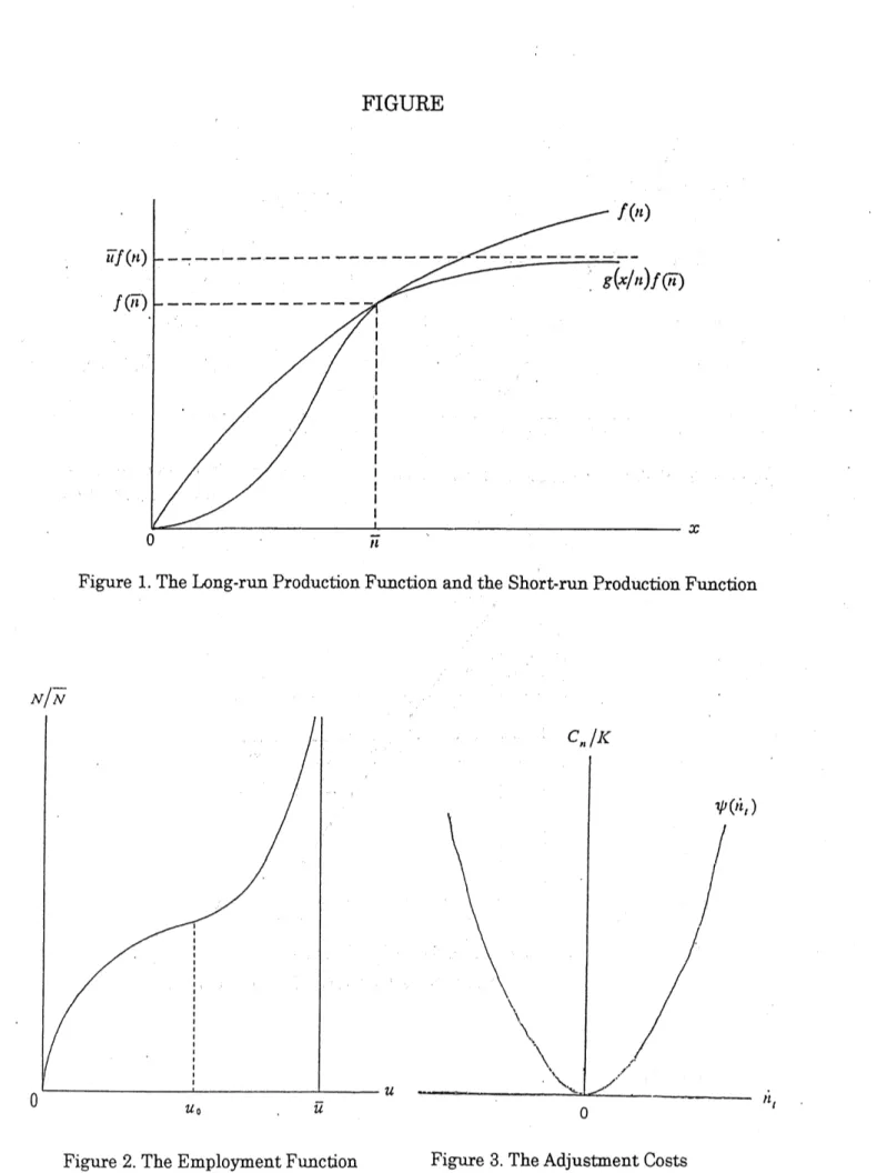
Figure 1 illustrates the relation between the long-run and short-run production

functions. As is explained above, the long-run production function shows

a

spectrum of

available $\mathrm{t}\epsilon \mathrm{c}\mathrm{h}\mathrm{n}\mathrm{i}\mathrm{q}\mathrm{u}\mathrm{e}\mathrm{s}$

as

the

relationshi-o

between the normal labor-capital,_$n$, and the

normaloutpul-capital ratio,$f(n)$. Suppose that the technique embodied inthe existing

capital stock is represented by $(\overline{\prime\iota},f(\overline{;\iota}))$

.

Then, the short-run production function

touches the long-run production function at $x=\overline{;\iota}$, since the existing capital stock is

normally utilized at thatpoint. Except thatpoint, the short-run$\sim \mathrm{o}\mathrm{r}\mathrm{o}\mathrm{d}\mathrm{u}\mathrm{c}\mathrm{t}\mathrm{i}\mathrm{o}\mathrm{n}\mathrm{f}\iota\iota \mathrm{n}\mathrm{c}\mathrm{t}\mathrm{i}\mathrm{o}\mathrm{n}$is

representsefficient frontier ofproduction.

In the following discussion,

_we

use

the inverse

function

of (4) for convenience. Let

us

define $u\equiv Y/\overline{\mathrm{Y}}$, which is called the rate of capital utilization. Then, the inverse

function of(4)maybewritten

as

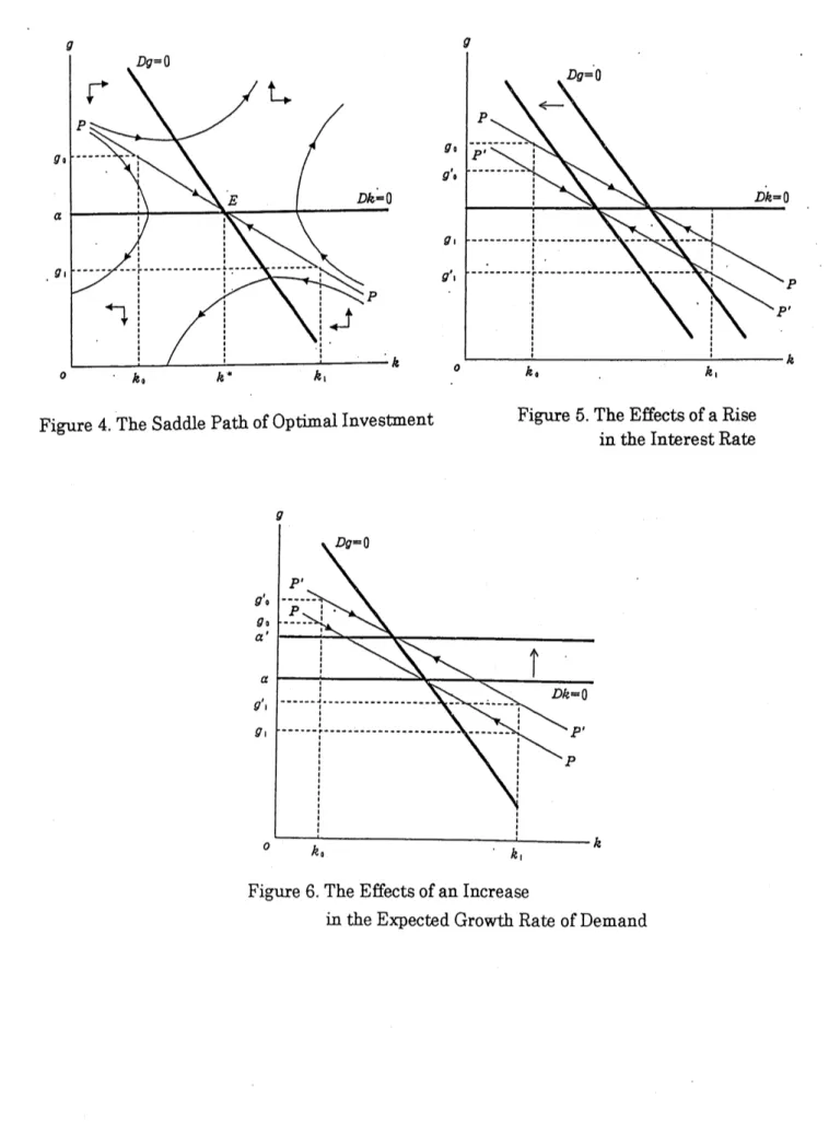
$\frac{N}{\overline{N}}=h(u)$

.

(6)

This function, which represents the required rate of employment for

a

given rate of utilization, is called the employment function in the following. The employment function $h(u)$ havethe followingproperties:

(a) $h(0)=0$ (b) $h’>0$ (c) $h(1)=1$

(d) There exists

some

real quantity $\overline{ll}>1$, such that $h(\overline{u})=\infty$ .

(e) _Thereexists

some

real quantity $u_{\mathrm{c}}<1$, such that:

if $u<u_{0}$, then $h”<0$; if $u=u_{0}$, then $h”=0$;

if $u>u_{0}$, then $h’>0$.

(f) $\frac{h(u)}{uh’(u)}=\frac{nf’(n)}{f(n)}$ ifandonlyif $n=1$

This function isillustratedby$\mathrm{F}\mathrm{i}_{3}\sigma \mathrm{u}\mathrm{r}\mathrm{e}2$.Itincreases withdecreasing rate for$u<u_{0}$, with

increasing rate for $u>u_{0}$, and $\mathrm{a}\mathrm{s}\mathrm{y}\mathrm{m}\mathrm{p}\mathrm{t}\mathrm{o}\mathrm{t}\mathrm{i}\mathrm{c}\mathrm{a}1_{1}^{1}\mathrm{y}$ approaches $\overline{u}>1$.

3. The Decisions of the Rate of

Capital

Utihzation under

Imperfect

$\mathrm{C}$

omp

etition

In this section,

we

examine how the imperfectly $\mathrm{c}\mathrm{o}\mathrm{m}\mathrm{p}\backslash$etitive firm determine its

output and prices, given the existingstock ofcapital and the technique embodied in it.

To determine the level of ourput, $Y$_, with given stock of capital is nothing but to

determine the rate of capital utilization, $u$ . So what we examine in this section is

reducedtothe determination of the rate ofcapital utilization and theprice ofoutput by

the imperfectly competitive firm. At a given $\dot{\mathrm{p}}$

oint of time, the representative firm under imperfect competition is faced with an expected demand

curve

with downward sloping. Let

us

denote the expected demand of the firm by $Y^{e}$and the price ofproduct by _$p$ . Then the expected

demand functionofthe firm is written

as

$Y^{e}=Ap^{-\eta}$, (7)

price elasticityof demand.A change in$A$ indicates

a

shift inthe expecteddemand

curve.

We

assume

$\eta$ tobeconstant inthe following.

Suppose that the firm determines output $\mathrm{Y}$ to be equal to the expected demand

$Y^{e}$

.

Then

we

can

rewrite (7) in theform ofinverse demandfunction

as

$p=( \frac{Y}{A})^{-\epsilon}=(\frac{Y}{K}\frac{K}{A})^{-\epsilon}=\{uf(n)k\}^{-\epsilon}$ (8)

where $\epsilon\equiv 1/\eta$ (theinverseofthe price elasticityofdemand) and $k\equiv K/A$(capitalper

unitofexpecteddemand).Thenormallabor-capitalratio $n$ isconstant in the short-run,

sincethe technologyembodiedin the existing capital isgiven. The short-runprofit $\Pi$ ofthe firm is given by

$\Pi=pY-7tN=[puf(n)-m(u)n]K$, (9)

where $W$ isthe money wage rate. The short-run decisionsofthe firm under imperfect

competitionistoset price and determine therateofcapitalutilization

so as

tomaximize

the profit, given the stock ofcapital and technology. Maximizing $\Pi$ withrespectto $u$

subject tothe$\mathrm{c}\mathrm{o}\mathrm{n}\mathrm{s}\mathrm{t}\iota \mathrm{a}\mathrm{i}\mathrm{n}\mathrm{t}(8)$ yields:

$(1-\epsilon)pf(n)=m’(l\mathit{1})n$ (10)

Thisequationhas

a

meaningfulsolution onlyif $e<1$ (or $\eta>1$).

So

the priceelasticity of demand for the representative must be greater than unity. In addition to this

condition, the secondordercondition forprofit

maximization

$\mathcal{E}+\frac{uh^{n}}{h’}>0$ (11)

must be satisfied. The second termofthe left-handside of(11) representsthe elasticity ofthe marginal employmentrate, $h’(u)$_, with _respectto capital utilization, $u$ . Let

us

denote itby $\sigma$

:

$\sigma\equiv\frac{uh^{f}}{h’}$. (12)

Then (11) is rewritten

as

$\epsilon+\sigma>0$ (13)

Thevalue of $\sigma$ may be eitherpositive

or

negative. Second order condition(13) implies

that

even

if it is negative, its absolute value cannot exceed $\epsilon$

.

This condition restricts

the degreeofincreasingreturnfor the short-run production function (5).

Substituting (8)_into (10),

we

have

$(1-\mathcal{E})\{llf(n)k\}^{-\mathit{5}}f(’\iota)=m^{l}(\iota r)n$. $\mathrm{j}$ . (14)

Since $k$ and $n$

are

constant in the short-run,

$\mathrm{t}_{}\mathrm{h}\mathrm{i}\mathrm{s}$equation determines _$u$

.

So _$u$ may

withrespect to $k$ is calculatedtobe

$\frac{k}{u}\frac{\partial u}{\partial k}=-\frac{\mathcal{E}}{\epsilon+\sigma}<0$

.

(15)

Thus $u$ is

a

decreasingfunction withrespect to $k$. This

means

that the rateofcapital

utilization, $u$, increases if thelevel ofexpecteddemand,$A$, risesunder

a

given stock of

capital, $K$.

The elasticityof $u$ with respectto $n$,

on

the otherhand, isshowntobe $\frac{n}{u}\neg\frac{Oll\neg}{\alpha\iota}=-\frac{1-(1-\epsilon)\theta}{\epsilon+\sigma}<0$, (16)

where $\theta$ isdefined

as

$\theta\equiv\frac{nf’(n)}{f(n)}$

.

(17)

Itrepresentstheelasticityof the long-run production function $f(n)$ withrespectto $n$,

and $0<\theta<1$ if the production function

satisfies

Inada’s conditions (3). Thus $u$ is

a

decreasing function with respect to $n$

.

It implies that, other things being equal,

a

higherlabor-capitalratioyields

a

lowerrate ofcapitalutilization.

The resultsobtained above

are

summarized

as

follows. In the short-run, giventhe values of $k$ and $n$, the rate of utilization, $u$, is determined by profit maximizing

condition (14), and then, the product price is determined by ghe _{inverse demand}

function (8). In other words, the short-run decisions ofthe representative firm under imperfect competitionis to determine the rate ofutilization and the price ofproduct at

eachpointoftime, given expecteddemand, capitalstock and $\mathrm{t}\mathrm{e}\mathrm{c}\mathrm{h}\mathrm{n}\mathrm{o}\mathrm{l}\mathrm{o}_{\Leftrightarrow}^{\sigma}\mathrm{y}$.

4. AModel of Investment Decisions and the Choice of

Technique

Inthe lastsection,

we

dealt withthe short-run decisions ofthefirm, giventhe stock of capital and technology. We

now

turn to the long-run decisions concerning with investment and $\mathrm{t}\mathrm{e}\mathrm{c}\mathrm{h}\mathrm{n}\mathrm{o}\mathrm{l}\mathrm{o}_{8}^{\sigma}\mathrm{y}$.

The investment decisions of the firm

are

made based

on

the expectations of about

demandand costs

over

the periods during which the newlyinstalledequipment will be used. So expectations for investment decisions may be characterized as long-run

expectations, differingfrom those for the $\mathrm{d}\mathrm{e}\mathrm{c}_{\sim}^{i}\mathrm{s}\mathrm{i}\mathrm{o}\mathrm{n}\mathrm{s}$ofcapitalutilization.

In order to make expectations about demand and costs central to investment

decisions,

we

follow the standard theory of investment decisions that emphasizes the

presence of costs to changing the $\mathrm{c}\mathrm{a}_{\wedge}\mathrm{o}\mathrm{i}\mathrm{t}\mathrm{a}1$ stock. In addition, however,

we assume

that

changes in techniques embodied in the capital stock also involve adjusrment costs. So

Let

us

first formulate the assumption about adjustment costs for investment. Following Hayashi (1983), adjustmentcosts per unit of investment

are

assumed torise

as a

function of $I_{t}/K_{t}$, which is denoted by $g‘$

.

in the following. Then, the total

adjustmentcosts $C_{t}$ is written$\mathrm{a}\mathrm{s}^{4}$

$C_{t}=\Phi(I_{t}/K_{t})I_{t}=\Phi(g_{t})I_{t}$, (18)

where $\Phi(g_{t})$ is the per-unit adjustment cost. This function is assumed to have the

followingproperties:

$\Phi(0)=0$, $\Phi’>0$_, $\Phi^{\pi}>0$

.

(19) Inother words, the perunit adjustmentcost increases

more

than proportionally

as

$g_{t}$

increases.

We

assume

the price ofcapital goods to be constant, putting it equal to unity for

convenience. Then, thetotalcostofinvestmentbecomes

as

$\{q_{\ell}+\Phi(g_{t})\}I_{t}=[\{1+\Phi(g_{t})\}g_{t}]K_{t}=\phi(g_{t})K_{t}$, (20)

where $\phi(g_{t})=\{1+\Phi(g_{t})\}g_{t}$

.

In view of(19),thisfunction has thefollowing properties:

$\phi(0)=0$, $\phi’>0$_, $\phi’’>0$. (21) If

we

$\mathrm{i}_{\epsilon}^{\sigma},\mathrm{n}\mathrm{o}\mathrm{r}\mathrm{e}$the depreciationofcapital,

we

have

$\dot{K}_{t}=g_{\ell}K_{\ell}$

.

(22)

Let

us

next consider adjustment costs accompanied by changes in the technique embodied in the capital stock. The technique embodied in the existing capital stock is

expressed by its normal labor-capital ratio $??_{t}.\cdot$ If capital is assumed to be completely malleable, labor-capital ratio $\mathrm{w}\mathrm{i}\mathrm{U}$ be adjusted instantaneously to changes in factor

prices. In reality, however, factor proportions

are

largely embodied in existing capital: technologyis putty-clay. In thiscase,the labor-capital ratio will notinstantaneouslyget

tothe optimal level responding to changes infactor prices. To take into accountof this

fact in

our

model, rather than explicitly allowingfor

a

putty-clay technology,

we

assume

that the firmfacescostofadjustingfactor

proportions.5

Then, whatthefirm

can

control in the short-run is not $n_{t}$ but its time derivative

$\dot{n}_{t}$. Denoting the firm’s control

variableby $s_{t}$,

we

have

$\dot{n}_{t}=S_{t}$

.

(23)

We

assume

that the costofadjusting the normallabor-capitalratio, $n_{t}$, depends

on

its

rate ofchange, $\dot{n}_{t}$, and the sizeofcapitalstock, $K_{t}$ ; specifically,

we

express it

as

$C_{n}=\psi(j_{l_{\ell}})K_{t}=\psi(s_{t})K_{t}$

.

(24)

Here, the function $\}^{\prime/(l\dot{l})}$

: representingthe adjustment cost per unit ofcapital has the following properties:

Inother words, the costofchanging $n_{\ell}$ increaaes with increasing rate

as

the degree of

itschangeincreases. The adjustmentcostsfunctionsatisfying (25)is showninFigure

3.

Taking into account the cost for investment (20) and the costfor changing factor

proportions(24),

we

can

expressthepresentvalueof the firm’slong-run profits

as

$V_{0}=\Gamma_{0}[p_{t}u_{t}f(n_{\ell})-W_{t}h(u_{t})n_{t}-\phi(g_{\ell})-\psi(s_{t})]K_{t}e^{-n}dt$, (26)

where

we

assume

the real rate of interest $r$ to be constant. In view ofthe inverse

demandfunction (8), theprice ofproductsisgiven by

$p_{\ell}=\{u_{t}f(n)k_{p}\}^{-\epsilon}$ (27)

and

as we

discussedinthe last section,the rate ofcapitalutilizationisgive by

$u_{\ell}=u(k_{t},n_{\ell})$, $u_{k}<0$, $u_{n}<0$ (28)

Here, $k_{t}$ isdefinedby

$k_{t} \equiv\frac{K_{\ell}}{A_{t}}$. (29)

Inthe $\mathrm{f}\mathrm{o}\mathrm{U}\mathrm{o}\mathrm{w}\mathrm{i}\mathrm{n}\mathrm{g}$ discussion,

we

assume

thatthe expected the firm expectsthe demand

fortheirproductat the givenpricelevel growsat

a

constantrate

a.

Therefore,

we

have

$A_{\ell}=A_{0}e^{a\ell}$ (80)

Takingthe time derivative ofequation (29) and substitutingfrom (30),

we

have

$\dot{k}_{\ell}=(g_{\ell}-\alpha)k_{t}$

.

(31)

To

sum

up, the problem ofinvestment decisions and the choiceoftechnique ofthe imperfectly competitive firm istomaximize

$V_{\mathrm{c}}= \int_{0}^{\infty}[p_{t}u_{t}f(n_{\ell})-W_{t}h(u_{\ell})n_{t}-\phi(g_{\ell})-\psi(s_{t})]k_{t}e^{-(r-\alpha\grave{)}\ell}dt$ , (32)

subject to the constraints

$\dot{k}_{t}=(g_{t}-\alpha)k_{t}$ (33)

$\dot{n}_{t}=s_{:}$, (34)

where $p_{t}$ is givenby (24).The variables that the firm

can

control

are

$g_{\ell}$ and $s_{t}$, while $k_{t}$ and

$n_{\ell}$

are

state variables.

To solve thisproblem,

we

set up the present-value Hamiltonian:

$H_{t}=e^{-(r- a)t}[\{p_{t}u_{\ell}f(n_{\ell})-W_{p}h(u_{t})fl.’-\phi(g_{t})-\psi(s_{t})\}k_{\ell}$

where $\lambda_{\ell}$ and

$\mu_{t}$

are

shadow prices of $k_{\ell}$ and

$n_{\ell}$, respectively. The first order

conditions for

a

maximumof $V_{0}$

are

$\lambda_{t}=\phi’(g_{t})$, (36a) $\mu_{\ell}=\psi’(s_{\ell})k_{t)}$ (36b) $\overline{\dot{\lambda}}_{\ell}=-$ (r-$g_{\ell}$)$\lambda_{t}-$ -$\{(1-\epsilon)p_{t}u_{t}f(n_{t})-W_{\ell}h(u_{t})n_{t}-\phi(g_{\ell})-\psi(s_{t})\}$, (36c) $\dot{\mu}_{t}=(r-\alpha)\mu_{t}-\{(1-\epsilon)p_{t}u_{f}j(n_{t})J’/-W_{t}h(u_{\ell})\}k_{t}$. (36d)

The transversalityconditions

are

$\lim_{tarrow\infty}k_{t}\lambda_{t}e^{-(r- a)\ell}=0$, $\lim_{tarrow\infty}n_{\ell}\mu_{t}e^{-(r-\alpha)t}=0$

.

(36e)

The system consisting of sixequations (33), (84), and $(3.5\mathrm{a})\sim(35\mathrm{d})$include sixvariables: $g_{t},$ $s_{t},$ $k_{\ell},$

$n.$”

$\hat{\nearrow}\vee\ell$ and

$\mu_{t}$. So it is complete. The solution of this system determines

the path of those variables. But the system is too complex to solve explicitly for the general solution. In the $\mathrm{f}\mathrm{o}\mathrm{U}\mathrm{o}\mathrm{w}\mathrm{i}\mathrm{n}\mathrm{g}$, therefore,

we

discuss investment decisions and the

choiceoftechnique separately by making

some

$\mathrm{s}\mathrm{i}\mathrm{m}\mathrm{p}\mathrm{l}\mathrm{i}\Phi \mathrm{i}\mathrm{n}\mathrm{g}$assumptions.

5. The Choice of

Technique

of the Firm under

Imperfect Competition

We first consider the choice$0\underline{\mathrm{f}}$technique of the firm. Equation(36b) shows that the

optimum rateof changeoflabor-capitalratio, $s_{t}$, determinesatwhichthe shadowprice

of labor per unit of capital equals the marginal adjustment cost of changing

labor-capitalratio. But, inviewof(36c), _{the shadow}price ofla\‘oorper unit ofcapital, $\mu_{t}$,

can

be expressed

as

follows:

$\mu_{t}=\int_{0}^{\Phi}e^{-(r-\alpha)(\tau-t)}\{(1-\vee p)p_{\sim}.u_{-}.f’(n_{\tau})-W_{\tau}h(u_{\mathrm{r}})\}k_{\tau}d\tau$ . (37)

Thisequation states that the valueof laborperunitofcapitalat

a

giventime equalsthe

$\mathrm{d}\mathrm{i}\mathrm{s}^{\backslash }\mathrm{c}\mathrm{o}\mathrm{u}\mathrm{n}\mathrm{t}\mathrm{e}\mathrm{d}$ value of its future marginal

revenue

products. Substituting this equation

into (36b),

we

have

$\psi’(s_{t})k_{t}=\ulcorner_{t}e^{-(r-\alpha \mathrm{X}^{\sim}-t)}.\{(1-\epsilon)p_{\mathrm{r}}u_{\mathrm{r}}f’(n_{\mathrm{r}})-W_{\tau}h(u_{\mathrm{r}})\}k_{\mathrm{r}}d\tau$ . (38)

At time $t,$ $k_{t}$ is given since it is

a

state variable. Therefore, this equation determines

$s_{t}$ if the firm’s$\mathrm{e}\mathrm{x}\iota$)

$\mathrm{e}\mathrm{c}\mathrm{t}\mathrm{a}\mathrm{t}\mathrm{i}\mathrm{o}\mathrm{n}$ofthe future marginal

revenue

productsis given. This result

implies that the firm’s expeclations about future demand and costs

are

crucial in the determination of $1\mathrm{a}\iota_{)\mathrm{o}\mathrm{r}- \mathrm{c}\mathrm{a}1)}\mathrm{i}\mathrm{t}\mathrm{a}1$ ratio if the adjustment costs for its changes

are

taking

intoaccount.

However, the discounted value of the future marginal productsof labor per unit of

wagesbut also

on

future valuesof $n$ and $k$. But, those future values

are

affected by

the levels of $s_{t}$ and $g_{t}$ to be determined at present. So, $s_{\ell}$ cannotbe determinedby equation (38) alone. It is determined simultaneously with other variables in the

complete system.

In orderto seek

a

$\mathrm{m}\mathrm{e}\mathrm{a}\mathrm{n}\mathrm{i}\mathrm{n}_{\epsilon}\sigma,\mathrm{f}\mathrm{u}1$ explanationfor the determination of thelabor-capital

ratio,

we

focus

on

the steady state of the complete system. Putting $\dot{k}_{t}=0$ in (33) and

$\dot{n}_{t}=0$ in (34),

we

have $g_{t}=\alpha$ and $s_{\ell}=0$ . Next, putting $\dot{j}_{\vee}.’=0$ in (36c) and

$\dot{\mu}_{t}=0$

in (36d), _{and substituting} ffom (35a) and (35b), respectively,

we

have the following

steadystate relationships:

$(1-\epsilon)puf(n)-Wh(u)n=\phi(\alpha)+(r-\alpha)\phi’(\alpha)$_{, (39)}

$(1-\epsilon)puf’(r?)-m(u)=0$

.

(40)

In viewof(27) and (28), the steady state values$0^{\underline{\{}}\wedge p$and $n$

are

determinedby

$p=\{uf(n)k\}^{-\epsilon}$ (41)

$u=u(k,n)$. (42)

Taking these relations into consideration, the steady-state values of $k$ and $n$

are

determined by (39) and (40). The wage rate, $W$_, the rate of interest, $r$, and the

expected rateofgrowth, $\alpha$,

are

given$\mathrm{e}\mathrm{x}\mathrm{o}_{\epsilon}^{\sigma},\mathrm{e}\mathrm{n}\mathrm{o}\mathrm{u}\mathrm{s}\mathrm{l}\mathrm{y}$.

If

we

use

equation(10)to substituoeout $\wedge p$ and $W$ inequation (40),

we

have $\underline{h(u)}\underline{nf’(n)}=$

(43)

$uh’(u)$ $f(n)$

Notice the $\mathrm{a}\mathrm{s}\mathrm{s}\mathrm{u}\mathrm{m}\mathrm{o}\mathrm{t}\mathrm{i}\mathrm{o}\mathrm{n}\mathrm{s}\wedge$that

were

made

on

the utilization function $h(u)$ in section 2.

SpecificaUy, assumption(f) states that(43)holds if and only if $u=1$. In otherwords, the

rate ofutilization is at the normal level in the steady stare. On thiscondition,

we can

rewrite (39) and (40)

as

follows:

$(1-\mathcal{E})pf(n)-Wn=\phi(\alpha)\perp(r-\alpha)\phi’(\alpha)$ (44)

$(1-\mathcal{E})pf’(n)-W=0$ (45)

Eliminating $p$ from thesetwo equations,

we

have

$\frac{f’(n)}{f(;\iota)-flf’(fl)}=\frac{W}{\phi(\alpha)\perp(r-\alpha)\phi’(\alpha)}$. (46)

Thisequation determines lhe normal $1\mathrm{a}\mathrm{b}_{\mathrm{o}\mathrm{r}- \mathrm{C}\mathrm{a}_{1})}\mathrm{i}\mathrm{t}\mathrm{a}1$ ratio, $n$, at the steady state, given

$W,$ $r$ and $\alpha$.

Calculating the effect ofa$\mathrm{c}\mathrm{h}\mathrm{a}\mathrm{n}_{3}^{\sigma}\mathrm{e}$in $W$

or

$r$

on

$n$ from equation(46),

we

have the

$\frac{Won\neg}{n\partial W}=\frac{f’(n)[f(n)-nf’(n)]}{nf(n)f’(n)}<0$ (47)

$\frac{1}{n}\frac{\partial n}{b}=-\frac{f’(n)[f(n)-nf’(n)]}{nf(n)f^{n}(n)}\frac{\phi’(\alpha)}{\phi(\alpha)+(r-\alpha)\phi(\alpha)}’>0$ (48)

Thus, the labor-capital ratio decreases with

an

increasein the wagerate, increases with

an

increase in the rate of interest. It should be noted that these results have been obtained from the comparison

of

steady states.

Since

the normal labor-capital ratio is fixed in the short-run in

our

model, it does not respond instantaneously to changes in the wage rate

or

interestrate. Corresponding to givenfactorprices, the optimum

labor-capital ratio is attained only at the steady state. But, it takes quite

a

long time for the

transition ffom

one

steady state to another. So changes in factor prices

can

lead to changes infactorproportionsonlyinthe long-run.

6. Investment Decisions

of

the Firm

under

Imperfect Competition

Let

us

nextconsiderinvestment decisionsofthe firm by assuming thatthe normal labor-capital ratio, $n$, is given. Since $\mathrm{c}\mathrm{h}\mathrm{a}\mathrm{n}_{\Leftrightarrow}^{\sigma}\mathrm{e}\mathrm{s}$ in the normal labor-capital ratio take

quite

a

longtime

as

is mentioned above,this simplifyingassumptionmay be justified.It should be noted, however, that the actual labor-capital ratio changes with the rate of capitalutilization

as

is alreadyexplainedinsection 2.

Withthis simplifyingassumption, investment decisionsof the firm isformulated

as

the problemofmaximizing

$V_{0}= \int_{0}^{\infty}[p_{t}u_{\ell}f(n)-W_{t}h(n_{t})n-\phi(g_{p})]k_{t}A_{0}e^{-(r-\alpha)\ell}dt$, (49) subject to

$\dot{k}_{t}=(g_{\ell}-\alpha)k_{t}$ . (50)

where the product price $p_{t}$ is given by (25), and the rate ofcapital utilization $u_{t}$ by

(26).

Since

the normal labor-capital ratio, $n$, is here assumed to be constant, those

equationsare written

as

$p_{t}=\{u_{t}f(r\iota)k_{t}\}^{-\epsilon}$ (51)

$ll_{\ell}=ll(k_{t})$ (52)

For analytical convenience,

_we

rewrite the objective function of the firm, (49), in

termsof therate ofreturn

on

capital definedby $\pi_{t}=(p_{t}Y_{f}-W_{t}N_{:})/q_{t}K_{t}$. Since weput

$\pi_{t}=\frac{p_{t}Y_{t}-W_{t}N_{t}}{K_{t}}=p_{t}u_{t}f(n)-W_{t}h(u_{t})n$

.

(53)

Substituting(51) and (10) into thisequationyields

$\pi_{t}=\frac{\epsilon+\xi-1}{\xi}\{u_{\ell}f(n)k_{t}\}^{-\epsilon}u_{t}f(n)$ , (54)

where $\xi$ isdefinedby

$\xi\equiv\frac{uh’}{h}$ (55)

Thus, the rate ofreturn, $\pi_{t}.$

’ is expressed

as

a

function of $u_{t},$ $k_{\ell}$ and _$n$. But, _$n$ is

assumedto be constantand $n_{\ell}$ is expressed

as a

function of

$k_{\ell}$ in view of(52). Hence, $\pi_{t}$ is reduced to

a

functionof $k_{t}$:

$\pi_{t}=\pi(k_{t})$

.

(56)

Calculatin$\mathrm{g}$ the elasticity of the rate ofreturn, $\pi_{t}$, with respect to $k_{\iota}$ from (53) and

(14)yields

$\omega(k_{t})\equiv-\frac{k_{t}}{\pi_{\ell}}\frac{d\pi_{t}}{dk_{t}}=\frac{\epsilon\xi}{\mathcal{E}+\xi-1}$

.

(57)

Inviewof(54), $\epsilon+\xi-1>0$ mustbe satisfiedif $\pi_{t}>0$.With thiscondition, therefore,

$\omega(k_{t}).>0$

.

This impliesthat $\pi_{:}$ is

a

decreasingfunction of $k_{t}$

.

Using (56),

we can

rewritethe objective function ofthefirm, (49),

as

follows:

$V_{0}=\Gamma_{0}[\pi(k_{t})-\phi(g_{t})]k_{t}A_{0}e^{-(r-\alpha)t}dt$ (58)

Thus, investment decisions ofthe firm become the problem ofdetermining $g_{t}$

so as

to

maximize (58) subjecttotheconstraint (50).

To solve this problem,

we

set up the presentvalue Hamiltonian:

$H_{t}=e^{-(r-\alpha)t}[\{\pi_{p}(k_{t})-\phi(g_{t})\}_{\mathcal{T}}.J_{\vee}(\ell g_{t}-\alpha)]k_{t^{\gamma}}$ (59)

where $)_{\bigvee_{\iota}}$ is the shadowprice of $k_{t}$

.

We put $A_{0}=1$ without the loss of generality.

Thefirstorder conditions for

a

maximum of $V_{0}$

are

$\lambda_{t}=\phi’(g_{t})$ (60a)

$\dot{\lambda}_{t}=J_{\vee}(tr-g_{\iota})-[\pi(k_{t})\{1-\omega(k_{\iota})\}-\phi(g_{t})]$ , (60b) where $\theta$ is $\mathrm{d}\mathrm{e}\iota_{1\mathrm{n}\mathrm{e}}^{\vee}\mathrm{d}$by (57)above. The transversality condit.ion is

$\lim_{tarrow\infty}k_{\ell}\phi’(g_{t})e^{-(r- a)t}=0$ (60c)

$\dot{g}_{t}=\frac{\phi’(g_{t})(r-0\sigma)\ell-[\pi(k_{t})\{1-\omega(k_{t})\}-\phi(g_{t})]}{\phi’(g_{t})}$

.

(61) Equations (61), (50) and (60c)characterize thefirm’s

investment

behavior.

Lt

us

analyze the system consisting of these equations by using phase diagram. The locusofpointswhere $\dot{g}_{t}=0$ satisfies

$\phi’(g)=\frac{\pi(k)\{1-\omega(k)\}-\phi(g)}{r-g}$ (62)

The slopeof this locus

on

$Okg$ plane iscalculated ffom this_equation

as

follows:

$\frac{dg}{dk}|_{\dot{g}=0}=\frac{\pi’(k)\{1-\omega(k)\}-\pi(k)\omega’(k)}{(r-g)\phi^{n}(g)}$

.

(63)

The second order condition for

a

maximug _of $(_{\backslash }49)$ implies that the right-hand side

expressionof(63)isnegative.Hence, _thelocusof $\dot{g}=0$ isdownwardsloping. Thelocus

ofpoints

where’

$\dot{k}_{\ell}=0$ satisfies

$g=\alpha$ (64)

This locus is

a

horizontal line

on

$Okg$ plane. The intersectionofthese loci denoted by $E(k,g^{*})$ _representsthe steady state.

In view of (61),

we

see

that $\dot{g}_{t}>0$ above the $\dot{g}=0$ line. and $\dot{g}.’<0$ below it. Similarly, it is obviousfrom (50)that $\dot{k}_{\ell}>0$ above the $\dot{k}=0$ line, and $\dot{k}<0$ below it.

Thus the direction ofthe movement ofthe system in eachphase becomes

as

Figure 4.

The steady staoe $E(k^{*},g^{*})$ becomes

a

saddle point, and there is

a

unique path that convergestoit. Though

we

omit the proof, it

can

be shown that

on

all otherpath, either

the optimalitycondition (61) eventuallyfails

or

the transversalitycondition (60c)_{is not}

satisfied.

The solution to the optimal investment decision $\dot{\mathrm{o}}\mathrm{f}$

the firm under imperfect

competitionis summarized bythe saddle path $PP$. Thisimpliesthat there is

a

unique

initial levelofinvestment per unit of capital, $g$, for each initial valueof $k$ (capitalper unitofexpecteddemand).Forinstance, if the initialcapitalper unitofexpecteddemand,

$k_{\mathrm{c}}$, is lower than its steady state value, $k$ , the optimal initial level ofinvestment per

unit ofcapif,$\mathrm{a}1,$

$g_{0}$, is higher than its steady state value, $g$

.

On the contrary, if the

initial capital per unit ofexpected demand, $k_{!},$ $\mathrm{i}.\mathrm{s}$

. higher than the steady state $\mathrm{v}\mathrm{a}\mathrm{l}\mathrm{u}\mathrm{e}_{2}$

$k$ _, the optimal investment $1$)$\mathrm{e}\mathrm{r}$ unit capital,

$g_{1}$, is lower than the steady state value,

point

on

the path $g$ and $k$ converges monotonically to $g^{*}$ and $k$ . Thisimplies that

$g$ decreases with $k$ monotonically. But,

as we

have shown before, $\pi$ is a decreasing

function of $k$. Therefore, _$g$ increases with $\pi$ monotonicaly. Therefore, the

investment per unit ofcapital, $g$, is

an

increasingfunction

of

the rate ofprofit, $\pi$.

Let

us

nextexamine how the rateofinterest, $r$, affectsthelevelof investmentper

unitofcapital, $g$. When $r$ rises, the $\dot{g}=0$ line will shift downwards

as

is shownin figure 5. Then, the saddle path $PP$ shifts down to $P’P’$_{. Therefore, for} any _given

initialvalueof $k,$ $g$ willdecreaae$\mathrm{r}\mathrm{e}\mathrm{s}\mathrm{p}\mathrm{o}\mathrm{n}\mathrm{d}\mathrm{i}\mathrm{n}_{\mathrm{a}}\sigma$ to

a

rise in _$r$. Forinstance, if the initial

value of $k$ is $k_{0}$, then _$g$ will decrease ffom $g_{0}$ to $\circ\sigma_{0}’$ . Thus, investmentper unitof

capitalchanges inverselywiththe rateofinterest.

Finally, we shall examine the effectof the expected growth rate ofdemand, $\alpha$, on

investment. When $\alpha$ increases, the $\dot{k}=0$ line willshiftupward

as

isshown in figure6. Then, the saddlepath $PP$ shiftup to $P’P’$_. Therefore, for anygiveninitialvalue of $k$_,

$g$ will increase responding to

an

increase in

a.

For instance, if the initial valueof $k$ is $k_{0}$, then _$g$ will increase from _{$g_{0}$} to $g_{0}’$

.

Thus, the expected growth rate of demand

has

a

positive influence

on

investmentper unitofcapital.

To summarize the above results, investment per unit of capital, $g$, is related

positivelyto $\pi$ and $\alpha$, and negatively to $r$

.

Thus, theinvestment function ofthe firm

under imperfect competition may be reprefented

as

$g_{t}=G(\pi_{t},r,\alpha)$, (65)

where

$\frac{\partial G}{o\pi_{t}}>0\neg$ ’

$\frac{\partial G}{\partial^{d}}<0$, $\frac{cG\neg}{\hat{c}\alpha}>0$

.

(66)

Aspecialfeature of this investment functionisthat in addition to the rate ofprofit and

the rate ofinterest, the expected growth rate of demand plays an importantrole

as

a

determinant of investment. The firms under imperfect competition make investment decisions based

on

expected future demands for their products. It is not price

expectations butquantity expectations. While the firm under perfectcompetition holds

price expectations, the firm under imperfectcompetitionholdsquantityexpectations in determining investment. The expected growth rate ofdemand, $a$, is

a

parameter that

represents the rate ofshifts in expected demand

curves over

time. Thisparameter may

$\mathrm{b}\mathrm{c})\mathrm{i}\mathrm{n}\mathrm{t}\mathrm{e}\mathrm{r}_{1})\mathrm{r}\mathrm{e}\mathrm{t}\mathrm{e}\mathrm{d}$ to correspond to what Keynes called ‘animal sprits’ ofentrepreneurs.

In the end,

we

should mention to the relation between the choice oftechnique and investment decisions. Aswehave

seen

in the lastsection, $\mathrm{c}\mathrm{h}\mathrm{a}\mathrm{n}_{\Leftrightarrow}^{\sigma}\mathrm{e}\mathrm{s}$ inthe wagerate, $W$,

or the rate ofinterest, $r$, will lead to $\mathrm{c}\mathrm{h}\mathrm{a}\mathrm{n}_{6}\sigma \mathrm{e}\mathrm{s}$ in the normal labor-capital ratio, $n$, in

obvious ffom (54), and thento changes ininvestment. To be

more

precise,

an

increase in

$W$ decreases $\pi$, and

so

tendstodecrease

$g$, while

an

increase in $r$ increases $\pi$, and

so

tends to increase$g$

.

It should be noted, however, that these indirect

effects

on

investmentthough the choice oftechnique will work only inthe long-run. Moreover,

as

for effects of $r$

on

investment, itsnegativeeffect discussed above willcertainly exceed

thepositive effectthrough the choiceoftechnique.

7.

Conclusions

In thispaper,

we

investigated investmentdecisions and the choice oftechnique of

the firm under imperfect competition.

Our

model has two special features. First,

we

analyzed firm’s investment decisions simultaneously with the choice oftechnique; and

second,

we

analyzed the behavior of imperfectly competitive firms. We distinguish

explicitly between the normal labor-capitalratio and the actuallabor-capitalratio. The

former is determinedbythe choice oftechnique of thefirm, _{and the latter by the}

raoe

_of utilizationofexisting capital. We assumed thatthenormallabor-capitalratiois fixedin

the short-run, and adjustment costs

are

needed for changing the ratio towards

an

optimallevel. So, in

our

model, adjustment costs

are

involved not only withinvestment

as

usual, but also with changes infactorproportions.

As for the choice oftechnique, the comparison ofsteady stateshas revealed that

a

rise in the wage rate decreases the labor-capital ratio, while

a

rise in the interestrate

increases its ratio. Theae results do not

seem

surprising. It should be noted, however, thatin

our

modelthe labor-capitalratioattains itsoptimallevelcorresponding tofactor prices only in the long-run. For, it takes quite

a

long time for the transition from

one

steady state toanother.

As for investment decisions,

we

have shown that the expected growth rate of

demandis

an

importantdeterminantofinvestment in

case

the firm isunder imperfect competition. This is due to the fact that the imperfectly competitive firm bases his investment decisions

on

quantity expectationsunlike the perfectlycompetitivefirm who bases his decisions on price expectations. The expected growth rate of demand may be

interpreted to correspond to Keynes’ animal spirits that reflect the state of long-run

expectationsof the firm.

Lastly,

we

have shown that the wage rate and the interest rate affect investment indirectly through their effects

on

the normal laboi-capital ratio. These indirect effects

NOTES

1.

Uzawa

(1972) gives

an

outline

of

the investment model

for

the

case

of the imperfect

competition. But he doesnot analyzethe modelin detail.

2. Okishio (1984) constructed

a

model of the simultaneous decisions of capital

utilization, investment and technique, and $\mathrm{d}\mathrm{i}_{\mathrm{b}}^{\neg}\mathrm{c}\mathrm{u}\mathrm{s}\mathrm{s}\mathrm{e}\mathrm{d}$

some

Keynes’s assertionsgiven

in ‘The

General

Theory’.This paper

owes

muchtohismodel. But his model deals with

only the

case

oftwo

or

three periods. Besides,

our

model focus

on

differentproblems

fromhis.

3. Most of the investment models presenoed

so

far do not differentiate between the long-run production function and the short-runproductionfunction. This distinction is made clear in the following literature: Okishio (1984), _Malinvaud (1989),

Malinvaud (1998).

4. This formulationofadjustment costsfollows Hayashi (1983).

5. Asimilarassumption ismadebyBlanchard (1997).

REFERENCES

Blanchard,

O.J.

(1997), “Medium Run.” $Bxooki_{Il}gsP_{\mathit{3}}pe\tau s$_odEconomicActivity2:

89-158.

Hayashi,F. (1983), “Tobin’sMarginal qandAverage q:ANeoclassicalInterpretation.” Econoaetfica50(1):213-224.

Malinvaud, E. (1983), “ProfitabilityandFactor Demands under Uncertainty.” De

EcoIlomist137: $2- 15$

.

Malinvaud, E. (1998), rDemandforInvestment,” Part 3, Chapter4inMacIoecoIlomic

Theorf.

VolumeA, $Ft\mathit{3}\Pi lewo\tau k$,Households$\mathit{3}JldFixJ\Pi S$, North-Holland:

352.402.

Okishio, N. (1984), “TheDecisions of NewInvestment, Technique, and theRate of

Utilization.” Kobe UniversityEconomicReview, Vol. 30: 15-32.

Uzawa, H (1972), _“TheTheoryofInvestment,” Chapter 10in TheTheoryofPxice.

FIGURE

Figure 1. TheLong-run Production FunctionandtheShort-run Production Functiion

$\lambda J/-\Lambda I$

$C/K$

Figure2. The EmploymentFunction $\mathrm{F}\mathrm{i}_{\mathrm{b}}\sigma \mathrm{u}\mathrm{r}\mathrm{e}3$

.

The Adjustment Costs

$\mathrm{F}\mathrm{i}_{\Leftrightarrow}^{\sigma}\mathrm{u}\mathrm{r}\mathrm{e}4$

.

The

Saddle

Path of Optimal Investment

Figure

5.

The Effects of

a

Rise

inthe Interest Rate

Figure

6.

The Effects of

an

Increase