Pulses,
kinks and fronts
in
the Gray-Scott model
$\mathrm{L}.\mathrm{A}$
.
PELETIERMathematicalInstitute, LeidenUniversity, Leiden, The Netherlands
1. Introduction
The Gray-Scott model represents what is called cubic autocatalysis [GS1-3], and is
given by the chemical reaction equations
Here $k_{1},$ $k_{2}$ and $k_{f}$
are
positive rate constants. In this lexturewe
discuss the situationin which the reactant $A$ is fed continuously into
an
unstirred reactor. The rate $\theta$ atwhich $A$ is supplied is assumed to be positive if the concentration $a$ of$A$ drops below
a
preassigned value $a_{0}$
,
and negative if it exceeds $a_{0}$.
Specifically, it is assumed that$\theta=k_{f}(a_{0}-a)$
.
The kinetics of this system leads to
a
pair ofordinary differential equations for theconcentrations $a(t)$ and $b(t)$ of, respectively, $A$ and $B$:
$\{$
$a’=-k_{1}ab^{2}+k_{f}(a_{0}-a)$, (l.la)
$b’=+k_{1}ab^{2}-k_{2}b$
.
(l.lb)For all values of the rate constants $k_{1},$ $k_{2}$ and $k_{f}$ the point
$(a, b)=(a_{0},0)$ is
a
stable node,and if
$\lambda^{\mathrm{d}}=^{\mathrm{e}\mathrm{f}}\frac{k_{1}k_{f}}{k_{2}}a_{0}^{2}>4$, (1.2)
there
are
two additional critical points, $P_{1}=(a_{1}, b_{1})$ and $P_{2}=(a_{2}, b_{2})$, numberedso
that $0<a_{2}<a_{1}<a_{0}$
.
The point $P_{1}$ isa
saddle and the point $P_{2}$ isa
spiral, which maybe stable
or
unstable. For $\lambda=4$ these two points coincide.In the absence ofstirring, the different concentrations depend not only
on
time $t$,but, due to diffusion, also
on
the location in the reactor. Assuminga
one-dimensionalgeometry, with spatial coordinate $x$, the Gray-Scott model then leads to the following
system of reaction-diffusion equations for the concentration profiles $a(x, t)$ and $b(x, t)$
Here $D_{A}$ and $D_{B}$
are
the diffusion coefficients ofthe chemicals $A$ and $B$.Proposed in
1983
by Gray and Scott [GS1], the Gray-Scott model has beenstud-ied
a
great deal,as a
simple polynomial mass-action model which has rich dynamics.For background information
we
refer to the papers of Horsthemke, Pearson, R\"ohricht,Swinney and Vastano [P,RH,VPI,$\mathrm{V}\mathrm{P}2$], in which bifurcation phenomena and Turing
patterns
are
discussed, and to Reynolds, Pearson&Ponce-Dawson
[RPP], in whichself-replicating patterns
are
analyzed. The Gray-Scott model is related to anotherau-tocatalytic reaction, the Brusselator [$\mathrm{N}\mathrm{P}$, p. 93]. We also mention here the
more
recentstudies by Nishiura&Ueyama [NU1,2]
on
self-replicating patterns andMimura&Na-gayama
[MN]on
the phenomenon of non-annihilation.More analytic studieshave been carried out by Merkin&Sadiq [MS], and Muratov
[M]. In papers by Doelman, Kaper
&Zegeling
[DKZ], Doelman, Gardner &Kaper[DGK] andDoelman, Eckhaus&Kaper [DEK],singularperturbation methods
were
usedto study the existence and stability of pulses under the assumption that $D_{B}/D_{A}\ll 1$
and $k_{f}/D_{A}\ll k_{2}/D_{B}$
.
.
We also mention the related work of Billingham&Needham [BN1-3] and Foquant
&Gallay [FG]. They discuss the existence andstability of travelling
waves
in the closedsystem ofchemical reactions
$A+nBarrow k(n+1)B$ with rate $kab^{n}$ for $n=1,2$, (1.4)
in the absence offeeding of the
chemical
$A$ and degeneration of the catalyst $B$.
In this lecture
we
discuss stationary Pulses and Kinks and their stability.Specifi-cally
we
shall obtain explicit expressions for such solutions if$\frac{k_{f}}{D_{A}}=\frac{k_{2}}{D_{B}}$, (1.5)
Regarding stability
we
find that if the diffusion coefficientsare
equal:$D_{A}=D_{B}$, (1.6)
the pulses
constructed
aboveare
unstable and the kinksare
stable.Inthis lecture
we
presentresults obtained incollaborations with$\mathrm{J}.\mathrm{K}$.
Hale (GeorgiaTech) and $\mathrm{W}.\mathrm{C}$
.
Troy (Pittsburgh) [HP1,2] and with Th. Gallay (Paris Sud) [GP].2. Dynamics
The
reaction diffusion
equations (1.3)can
be simplified by introducing thedimen-sionless variables
$u= \frac{a}{a_{0}}$ $v= \frac{b}{a_{0}}$
and the
dimensionless
constants$A= \frac{k_{f}}{k_{1}a_{0}^{2}}$ $B= \frac{k_{2}}{k_{1}a_{0}^{2}}$ and $d= \frac{D_{B}}{D_{A}}$
.
(2.2)When
we
drop then drop the tildes again,we
obtain the system of equations,$\{$
$u_{t}=u_{xx}-uv^{2}+A(1-u)$ (2.3a)
$x\in \mathrm{R}$
,
$t>0$.
$v_{t}=dv_{xx}+uv^{2}-Bv$ (2.3b)
We
assume
that initiallythe concentration profiles $a(x, 0)$ and $b(x, 0)$are
given, andwe
set$u(x, 0)=u_{0}(x)$ and $v(x, 0)=v_{0}(x)$ for $x\in \mathrm{R}$, (2.3c)
where, in view of the definition of$u$ and $v$, the initial data $u_{0}$ and $v_{0}$
are
assumed to benonnegative functions.
We make the following observations: Let $(u, v)$ be
a
solutionof the system (2.3) inthe strip $S_{T}=\{(x, t) : x\in \mathrm{R}, 0\leq t<T\}$
.
Then(1) $u(x, t)\geq 0$ for $(x, t)\in S_{T}$.
This follows immediately because $u=0$ is
a
sub-solutionof equation (2.3a).(2) $v(x, t)\geq 0$ for $(x, t)\in S_{T}$,
because $v=0$ is
a
solution of equation (2.3b).(3) $u(x, t)\leq 1$ for $(x, i)\in S_{T}$,
because $u=1$ is
a
super-solution of equation (2.3a).There exists
a
constant $M>0$ which dependson
the initial data $u_{0}$ and $v_{0}$, such that(4) $v(x, t)\leq M$ for $(x, t)\in S_{T}$.
The proofof this upper bound is
more
delicate anduses
ideas ofCollet&Xin [CX] (see[GP]$)$.
3. Stationary solutions
For stationary solutions of (2.3)
we can
further reduce the number ofparametersby introducing
new
independent and dependent variables:and the constants
$\lambda=\frac{A}{B^{2}}$ and $\gamma=Bd$
.
(3.2)The constant $\lambda$ in (3.2) is the
same as
theone
defined in (1.2). These scalings yielda
system of equations which involves only two parameters: $\lambda$ and
$\gamma$:
$\{$
$u”=uv^{2}-\lambda(1-u)$, (3.3a)
$\gamma v’’=v-uv^{2}$
.
(3.3b)If$\lambda<4$ the only constant solutionis $P_{0}=(1,0)$ and if $\lambda>4$ the constant solutions
are
$P_{0}$, as
wellas
$P_{1}$ and $P_{2}$.
In [HPTI] it
was
shown that it is possible to obtain explicit pulse and kink typesolutions of Problem (2.3) if
$\lambda\gamma=1$ and $\lambda>4$ (or $0< \gamma<\frac{1}{4}$). (3.4)
This
range
of $\lambda$ values coincides with therange
of values for which the null-clines alongwhich $u”$ and $v”$ vanish intersect. That is, if
we
write$\mathrm{K}=\{(u, v) : u’’=0\}$ and $\mathrm{L}=\{(u, v) : v’’=0\}$
,
(3.5)then $K\cap L\neq\emptyset$ if and only if $\lambda>4$ (see Fig. 1).
(a) $\lambda<4(\lambda=1)$ (b) $\lambda>4(\lambda=8)$
Fig. 1. Null-clines
In [DKZ], [DGK] and [DEK] the existence of solutions is investigated under the
assump-tion that $d$ is
small and
that $\lambda\gamma<<1$.
Thus, Figure ladescribes
the relative positionof the null-clines in these
papers.
In this paper, the null-clines intersect and Figure lbapplies.
Theorem 3.1. Let $\lambda$ and
$\gamma$
sa
$tis\theta(3.4)$, and $0< \gamma<\frac{2}{9}$,
then the pair offunctions$u(x)$ and $v(x)$ given by
$u(x)=1- \frac{3\gamma}{1+Q\cosh(x/\sqrt{\gamma})}$, $v(x)= \frac{3}{1+Q\cosh(x/\sqrt{\gamma})}$, (3.6)
in which $Q=\sqrt{1-\frac{9\gamma}{2}}$
,
isa
homoclinic $sol$ution ofProblem (3.3).Theorem 3.2. Let $\lambda$ and
$\gamma$
sa
tisff
(3.4), and $\frac{2}{9}<\gamma<\frac{1}{4}$,
then the pair offunctions$u(x)$ and$v(x)$ given by
$u(x)= \frac{1-\omega}{2}+\frac{a\gamma}{1+b\cosh(cx)}$, $v(x)= \frac{1+\omega}{2\gamma}-\frac{a}{1+b\cosh(cx)}$, (3.7a)
in which
$a= \frac{3}{\gamma}\frac{\omega(1+\omega)}{1+3\omega}$, $b= \frac{\sqrt{1-3\omega}}{1+3\omega}$, $c= \frac{\sqrt{\omega(1+\omega)}}{\gamma\sqrt{2}}$, (3.7b)
$is$
a
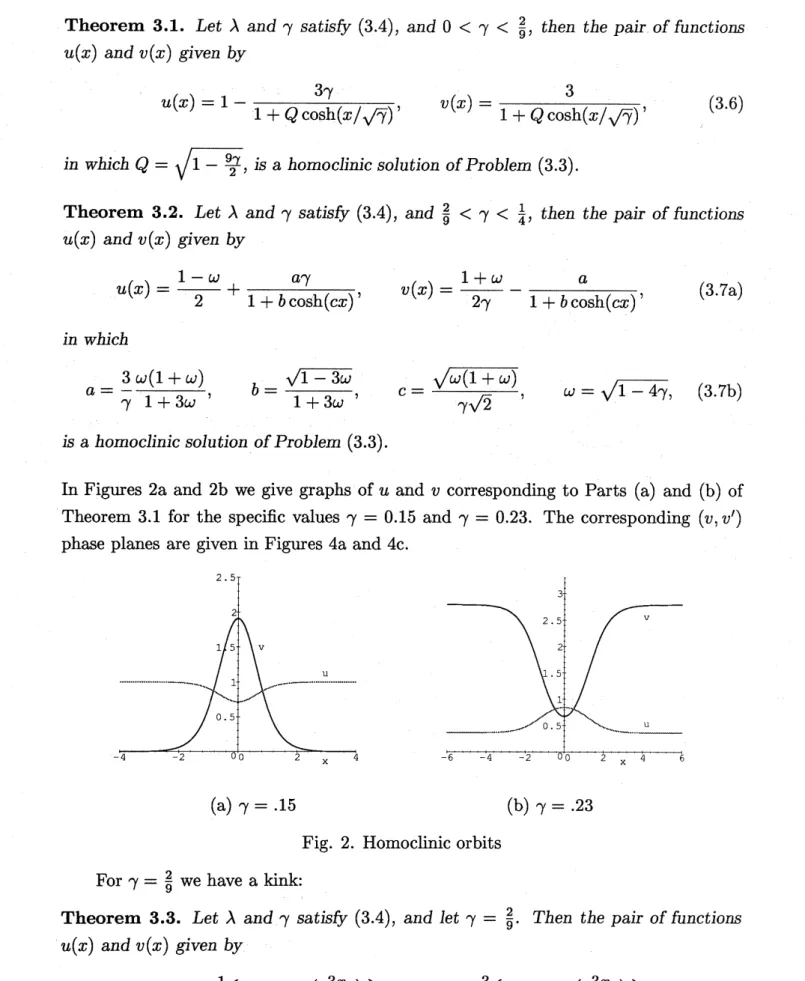
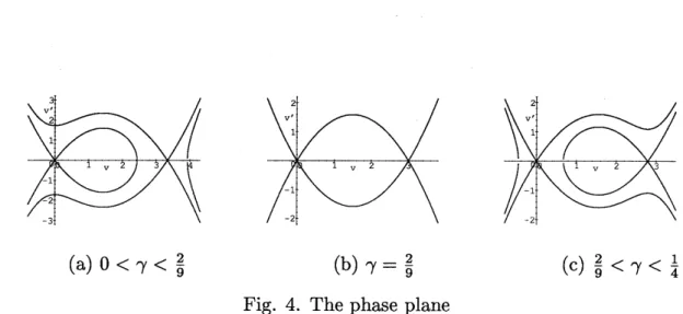
$hom$oclin$icsol\mathrm{u}$tion of Problem (3.3).In Figures $2\mathrm{a}$ and $2\mathrm{b}$
we
give graphs of$u$ and $v$ corresponding to Parts (a) and (b) of
Theorem 3.1 for the specific values $\gamma=0.15$ and $\gamma=0.23$
.
The corresponding $(v, v’)$phase planes
are
given in Figures $4\mathrm{a}$ and $4\mathrm{c}$.
(a) $\gamma=.15$ (b) $\gamma=.23$
Fig. 2. Homoclinic orbits
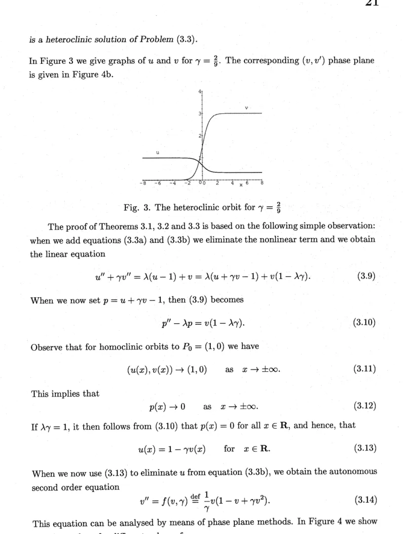
For $\gamma=\frac{2}{9}$
we
havea
kink:Theorem 3.3. Let $\lambda$ and
$\gamma$
sa
$tis6^{r}(3.4)$, and let $\gamma=\frac{2}{9}$.
Then the pair of functions$u(x)$ and$v(x)$ given by
$is$
a
heteroclinic $sol\mathrm{u}$tion of Problem (3.3).InFigure 3
we
give graphs of$u$ and $v$ for $\gamma=\frac{2}{9}$. The corresponding $(v, v’)$ phase planeis given in Figure $4\mathrm{b}$
.
Fig. 3. The heteroclinic orbit for $\gamma=\frac{2}{9}$
The proof of Theorems 3.1, 3.2 and 3.3is based
on
the following simple observation:when
we
add equations (3.3a) and (3.3b)we
eliminate the nonlinear term andwe
obtainthe linear equation
$u”+\gamma v’’=\lambda(u-1)+v=\lambda(u+\gamma v-1)+v(1-\lambda\gamma)$
.
(3.9)When
we now
set $p=u+\gamma v-1$, then (3.9) becomes$p^{j\prime}-\lambda p=v(1-\lambda\gamma)$
.
(3.10)Observe that for homoclinic orbits to $P_{0}=(1,0)$
we
have$(u(x), v(x))arrow(1,0)$
as
$xarrow\pm\infty$.
(3.11)This implies that
$p(x)arrow 0$
as
$xarrow\pm\infty$.
(3.12)If $\lambda\gamma=1$
,
it then follows from (3.10) that $p(x)=0$ for all $x\in \mathrm{R}$, and hence, that$u(x)=1-\gamma v(x)$ for $x\in \mathrm{R}$
.
(3.13)When
we now
use
(3.13) to eliminate$u$from equation (3.3b),we
obtainthe autonomoussecond
order equation$v”=f(v, \gamma)^{\mathrm{d}}=^{\mathrm{e}\mathrm{f}}\frac{1}{\gamma}v(1-v+\gamma v^{2})$
.
(3.14)This equation
can
be analysed bymeans
of phase plane methods. In Figure 4we
show(a) $0< \gamma<\frac{2}{9}$ (b) $\gamma=\frac{2}{9}$ (c) $\frac{2}{9}<\gamma<\frac{1}{4}$
Fig. 4. The phase plane
The proofs of Theorems 3.1-3
can now
be given by elemetary computations.In additionto the homoclinic and heteroclinic orbits
we
obtaina
family ofperiodicsolutions:
For every $\gamma\in(0,\frac{1}{4})$ Problem (3.3) has $a$ one-parameter family
of
periodic orbits when$\lambda\gamma=1$
.
These periodic orbits accumulate
on
one
of the homoclinic orbits,or
the heteroclinicorbits, when their periods tend to infinity [VF].
4. General properties of pulses
Let $(u, v)$ be
a
pulse type solution of (3.3) such that$(u(x), v(x))arrow(1,0)$
as
$xarrow\pm\infty$. (4.1)Then
we can
make the following observations.(a) We begin with
an
upper
bound for $u$:$u(x)<1$ for $x\in \mathrm{R}$
.
(4.2)Proof. We write equation (3.3a)
as
$u”-v^{2}u=-\lambda(1-u)$
on
R. (4.2)Suppose that $\max_{\mathrm{R}}u>1$
.
Then $u$ attains its maximum ata
point $x_{0}\in$ R. Plainly,at $x_{0}$ the left hand side of (4.2) is negative, and the right hand side is positive;
a
contradiction. Therefore $u\leq 1$
on
$\mathrm{R}$,so
thatThus, by the strong maximum principle, $u<1$
on
R.(b) Property (a) enables
us
toprove
that$v(x)>0$ for $x\in \mathrm{R}$
.
(4.4)Proof. We write equation (3.3b)
as
$\gamma v’’-v=-uv^{2}\leq 0$
on
$\mathrm{R}$, (4.5)and
we see
that (4.4) holds by the strong maximum principle.(c) We have
$\lambda\gamma\leq 1(\geq 1)$ $\Rightarrow$ $u+\gamma v<1(>1)$
.
(4.6)This is
an
immediate consequence of Property (b), equation (3.7) and the strongmax-imum principle.
(d) In the region$\lambda\gamma<1$ there
can
only exist homoclinic orbits to $(u, v)=(1,0)if \gamma<\frac{1}{4}$.
Proof. Plainly, the maximum of $v$ is attained at
an
interior point; letus
denote it by$x_{0}$
.
Then $v”(x_{0})\leq 0$.
Thismeans
that$v> \frac{1}{u}$ at $x_{0}$
.
(4.7a)Because, by Property (c),
$v< \frac{1}{\gamma}(1-u)$ at $x_{0}$, (4.7b)
The conditions (4.7a) and (4.7b)
can
only be reconciled if$\gamma<\frac{1}{4}$.
5.
Continuation
The branch of exact solutions $\Sigma=\{(\lambda, \gamma) : 0<\gamma<\frac{1}{4}\}$
can
be takenas a
startingpoint of
a continuation
to values of $(\lambda, \gamma)$ in the neighbourhood of $\Sigma$.
This has beendone in [HPTI], both for the homoclinic and the heteroclinic orbits.
Below
we
give an outline of the argument for the heteroclinic orbits. It uses theImplicit Function theorem and is
an
application Lin’s method [L]. We start from theexplicit kink at
$(\lambda, \gamma)=(\lambda_{0}, \gamma_{0})$ where $\lambda_{0}=\frac{9}{2}$ $\gamma_{0}=\frac{2}{9}$
.
(5.1)We denote this kink by
where $v_{0}$ is given in Theorem 3.3.
We first reformulate the problem. We introduce
a
small parameter $\epsilon$ and smallperturbations of$\lambda_{0},$ $\gamma_{0},$ $p=0$ and $v_{0}$:
$\lambda\gamma=1+\epsilon$, $p=\epsilon r$, $v=v_{0}+w$
.
(5.3)When
we
substitute these expressions into the equations for $p$ and $v$we
obtain for $r$and $w$ the system
Here
$q_{0}=f_{v}(0, v_{0}, \gamma_{0})=\frac{1}{\gamma_{0}}(1-2v_{0}+3\gamma_{0}v_{0}^{2})arrow\frac{1}{\gamma_{0}}$
as
$xarrow\pm\infty$. (5.5)We shall prove the following theorem:
Theorem 5.1. (a) There esists
a
smootharc
$C=\{(\lambda(\epsilon), \gamma(\epsilon)) : |\epsilon|<\epsilon_{0}\}$, $(\epsilon_{0}>0)$
ofheteroclin$ic$ orbits $(u(\epsilon), v(\epsilon))$ of Problem (3.3) such that
$(\lambda(\epsilon),\gamma(\epsilon))arrow(\lambda_{0,\gamma_{0}})$ and $(u(\epsilon), v(\epsilon))arrow(u_{0}, v_{0})$
as
$\epsilonarrow 0$,(b) The
arc
$C$ intersects thecurve
$\{\lambda\gamma=1\}$ underan
angle given by$\frac{d\lambda}{d\gamma}|_{C}(\lambda_{0}, \gamma_{0})=\frac{10-\pi^{2}}{\pi^{2}-7}$
.
$\frac{\lambda_{0}}{\gamma_{0}}=0.920165\ldots$.
(5.6)Here the
convergence
is in the space of$bo$un
$ded$ continouous functionson
R.We proceed in
a
series of steps.$\mathrm{S}\mathrm{t}\mathrm{e}_{-}\mathrm{p}1$
.
We choose and element $w$ inthe set $C_{B}(\mathrm{R})$ ofcontinuous functionson
$\mathrm{R}$ whichare
uniformly bounded. With this function $w$we
can
solveequation (5.4a) uniquely;we
denote its solution by
$r=H(\gamma, \epsilon)(v_{0}+w)$,
so
that $r_{0}=H(\gamma_{0},0)(v_{0})$.
(5.7)We put this solution into the second equation (5.4b). This yields
an
equation of theform
in which $q_{0}(x)$ has been defined in (5.5). Before
we can
solve this equation,we
need toinspect the eigenvalue problem
$-..y”+q_{0}(x)y=\kappa y$
on
R. (5.9)$\mathrm{S}\mathrm{t}\mathrm{e}_{\mathrm{D}}2$
.
Equation (5.9) hasa
zero
eigenvalue with corresponding eigenfunction $v_{0}’(x)$, sothat if $y$ is
a
solution of equation (5.8), thenso
is $y+tv_{0}’$ for any$t\in \mathrm{R}$
.
We thereforesplit the space $C_{B}(\mathrm{R})$:
$C_{B}(\mathrm{R})=\mathrm{Y}_{0}\oplus \mathrm{Y}_{1}$
,
(5.10a)where
$Y_{0}=\{tv_{0}’ : t\in \mathrm{R}\}$ and $\mathrm{Y}_{1}=\{y\in..C_{B} : (y, v_{0}’)=0\}$
.
(5.10b)It iswellknown that if$g\in \mathrm{Y}_{1}$, thenthere exists
a
unique solution$y\in \mathrm{Y}_{1}$ of theequation(5.8).
Step 3. We define the projection operators
$P:C_{B}arrow \mathrm{Y}_{0}$ and $1-P:..C_{B}arrow Y_{1}$, (5.11)
and solve the equation
$-y”+q_{0}(x)y=(I-P)h(\epsilon H(\gamma, \epsilon)(v_{0}+w),$ $w,$$\gamma)$
on
R. (5.12)We denote the unique solution in $\mathrm{Y}_{1}$ by
$y^{\mathrm{d}}=^{\mathrm{e}\mathrm{f}}\mathcal{T}(w, \gamma, \epsilon)\in \mathrm{Y}_{1}$
.
(5.13)Step 4. We prove that for
$|\gamma-\gamma_{0}|+|\epsilon|<\mathcal{U}$,
where $\nu$ is
a
smallnumber, the operator$\mathcal{T}$in equation (5.13) has
a
fixed point $w^{*}(\gamma, \epsilon)$.
This solution will be
a
solution of the originatproblem if$Ph(\epsilon H(\gamma, \epsilon)(v_{0}+w^{*}),$$w^{*},$$\gamma)=0$, (5.14)
or, in view of the definition of the projection$P$
,
$\mathcal{G}(\gamma, \epsilon)^{\mathrm{d}}=^{\mathrm{e}\mathrm{f}}\int_{\mathrm{R}}h(\epsilon H(\gamma, \epsilon)(v_{0}+w^{*}),$$w^{*},\gamma)v_{0}’dx=0$
.
(5.15)Because $\mathcal{G}$ is
differentiable near
$(\gamma_{0},0)$we
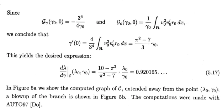
haveSince
$\mathcal{G}_{\gamma}(\gamma_{0},0)=-\frac{3^{4}}{4\gamma_{0}}$ and
$\mathcal{G}_{\epsilon}(\gamma_{0},0)=\frac{1}{\gamma_{0}}\int_{\mathrm{R}}v_{0}^{2}v_{0}’r_{0}dx$,
we
conclude that$\gamma’(0)=\frac{4}{3^{4}}\int_{\mathrm{R}}v_{0}^{2}v_{0}’r_{0}dx=\frac{\pi^{2}-7}{3}\gamma_{0}$
.
This yields the desired expression:
$\frac{d\lambda}{d\gamma}|_{C}(\lambda_{0}, \gamma_{0})=\frac{10-\pi^{2}}{\pi^{2}-7}$
.
$\frac{\lambda_{0}}{\gamma_{0}}=0.920165\ldots$. (5.17)InFigure $5\mathrm{a}$
we
show the computedgraph of$C$, extendedaway from the point $(\lambda_{0}, \gamma_{0})$;
a
blowup of the branch is shown in $\mathrm{F}^{1}\mathrm{i}\mathrm{g}\mathrm{u}\mathrm{r}\mathrm{e}5\mathrm{b}$.
The computationswere
made with
AUTO97 [Do].
(a) The global branch (b) Blowup
near
$(\lambda_{0}, \gamma_{0})$Fig. 5. The branch $C$ ofheteroclinic orbits
We conclude with
a
few remarks about the stability of the pulses and kinks whichweconstructed. When the two diffusion coefficients$D_{A}$ and$D_{B}$
are
equal, itis stillpossibleto decouple the two equations, and
so
analyse the spectrum around the solutionson
thebranch $\{\lambda\gamma=1 : \lambda>4\}$
,
using well known results about the second order equation(3.14). It turns out that thespectrum ofthe kinklies entirelyin the negativehalfplane,
implying local stability [He], and that the spectrum of the pulses has eigenvalues with
both positive and negative real part, implying instability [HPT2].
References
[BN1] Billingham, J.,
&D.J.
Needham The development oftravelling waves in quadratic and cubicauiocatalysis with unequal diffusion rates. I. Permanent form travelling waves, Phil. Trans.
Roy. Soc. London A 334 (1991) 1-24.
[BN2] Billingham, J.,
&D.J.
Needham, The development of travelling wavesin quadratic and cubic autocaialysiswith unequaldiffusion rates. II. An initial-valueproblem withanimmobilizedor[BN3] Billingham, J., &D.J. Needham, Thedevelopment oftravellingwaves in quadraticand cubic
autocatalysiswithunequaldiffusion rates. III. Large timedevelopmentin quadratic
autocatal-ysis, Quart. Appl. Math. 50 (1992) 343-372.
[CX] Collet, P.
&J.
Xin, Global existence and large time asymptotic bounds of$L^{\infty}$ solutions ofthermal diffusive combustion systems on $\mathrm{R}^{n}$, Ann. Scuola Norm. Sup. Pisa Cl. Sci. 23 (1996), 625-642.
[D] Devaney, R., Blue sky catasirophies in reversible and Hamiltonian systems, Indiana Univ.
Math. J. 26 (1977) 247-263.
[Do] Doedel,E.J. et.al., AUTO97: Continuationand Bifurcation Software for Ordinary Differential Equations (with HomCont), available by ftp from
$\mathrm{f}\mathrm{t}\mathrm{p}://\mathrm{f}\mathrm{t}\mathrm{p}.\mathrm{c}\mathrm{s}.\mathrm{c}\mathrm{o}\mathrm{n}\mathrm{c}\mathrm{o}\mathrm{r}\mathrm{d}\mathrm{i}\mathrm{a}.\mathrm{c}\mathrm{a}/\mathrm{p}\mathrm{u}\mathrm{b}/\mathrm{d}\mathrm{o}\mathrm{e}\mathrm{d}\mathrm{e}\mathrm{l}/\mathrm{a}\mathrm{u}\mathrm{t}\mathrm{o},(1997)$ .
[DF] Dockery, J.D.
&R.J.
Field, Numerical evidence ofstationary breathing concentrationpatternsin the Oregonator with equal diffusivities, Preprint, 1998.
[DEK] Doelman, A., W. Eckhaus
&T.J.
Kaper, Slowly-modulated two-pulsesolutions in the Gray-Scott model II.. geometric theory, bifurcations and splitting dynamics, to appear in SIAM J. Appl. Math., 2000.[DGK] Doelman, A., R.A. Gardner
&T.J.
Kaper, A stability index analysis of l-D patterns of theGray-Scott model, to appear inMemoirs of the American Mathematical Society, 1998.
[DKZ] Doelman, A., T.J. Kaper
&P.A.
Zegeling, Pattern formation in the l-D Gray-Scott model, Nonlinearity 10 (1997) 523-563.[FG] Focant, S.
&Th.
Gallay, Existence and stability of propagating fronts for an anutocatalyticreaction-diffusion system, Physica D120 (1998) 346-368.
.
$\mathrm{t}$[GP] Gallay, Th.
&L.A.
Peletier, Notes.[GS1] Gray, P.
&S.K.
Scott, Autocatalyiicreactions in the isothermal continuous stirred tank reactor: isolas and other forms ofmuliistability, Chem. Engg. Sci. 38 (1983) 29-43.[GS2] Gray, P.
&S.K.
Scott, Autocatalyticreactionsinthe isotheimal continuousstirred tank reactor: oscillations and instabilities in the system $A+2Barrow 3B,$ B $arrow C$, Chem. Engg. Sci. 39 (1984) 1087-1097.[GS3] Gray, P.
&S.K.
Scott, Sustainedoscillations and otherexoticpatterns of$beha\iota^{\gamma}io\mathrm{r}$inisothermalreactions, J. Phys. Chem. 89 (1985), 22-32.
[H1] Hale, J.K., Ordinary differential equations, Wiley, New York, 1969.
[H2] Hale, J.K., Introduction to dynamic bifurcation, In Bifurcaiion theory and applications (Ed. L. Salvadori), p 106-151, Springer Lecture Notes $\#$ 1057, Springer Verlag, Berlin, 1984.
[He] Henry, D.,
Geometric
theory ofsemilinear para
bolic equations, Lecture Notes inMathe-matics 840, Springer Verlag, 1981.
[HPTI] Hale, J.K., L.A. Peletier
&W.C.
Troy, Exact homoclinic and heteroclinic solutions of the Gray-Scott model forautocatalysis, to appear in SIAM J. Appl. Math. 2000.[HPT2] Hale, J.K., L.A. Peletier&W.C. Roy, Stability and instabilityin the Gray-Scott model: the
case ofequal diffusivities, Appl. Math. Lett. 12 (1999) 59-65.
[LS] Lee, K.J.
&H.L.
Swinney, Lamellar structures and self-replicatingspotsin areaction-diffusionsystem, Phys. Rev. E. 51 (1995) 1899-1915.
[L] Lin, X.-B., Using$Mel’\dot{m}ko1^{\Gamma}’ S$methodto solveSil’nikov’sproblems,Proc. Roy. Soc. Edinburgh
116A (1990) 295-325.
[MN] Mimura, M.
&M.
Nagayama, Nonannihilation dynamics in an exothermic reaction-diffusion system with mono-stable excitability, Chaos 7 (1997) 817-826.[MO] Muratov, C.B.
&V.V.
Osipov, Spike autosolutions in the Gray-Scott model, Preprint.[MS] Merkin, J.H. &M.A. Sadiq, Thepropagation oftravellingwaves in anopen cubic autocatalyiic chemicalsystem, IMA J. Appl. Math. 57 (1996) 273-309,
[NP] Nicolis,G.
&I.
Prigogine, Self-organisation innonequilibriumsystems,Wiley, NewYork, 1977.[NU1] Nishiura, Y. &D.Ueyama, Spatio-iemporal chaos for the Gray-Scott model, Preprint.
[NU2] Nishiura, Y. &D.Ueyama, A skeleton structure of self-replicating dynamics, Physica D, 130 (1999) 73-104.
[P] Pearson, J.E., Complexpatternsin a simple system, Science 216 (1993) 189-192.
[BPP] Reynolds, W.N., J.E. Pearson
&S.
Ponce-Dawson, Dynamics ofself-replicatingpatterns inreaction diffusion systems, Phys. Rev. Lett. 72 (1994) 2797-2800.
[RH] R\"oricht, B,
&W.
Horsthemke, A bifurcation sequence to stationary spatial patterns in anonuniform chemical model$syste\pi \mathrm{J}$ withequaldiffusion coefficients,J. Chem. Phys. 94 (1991)
4421-4426.
[VF] Vanderbouwhede, A. &B. Fiedler, $Homoclim\dot{c}$period blowup in reversible and $conse\mathrm{r}\iota^{r}\mathrm{a}ti\mathrm{v}e$
systems, Z. angew. Math. Phys. 48 (1992) 292-318.
[VP1] Vastano, J.A., J.E. Pearson, W. Horsthemke&H.L. Swinney, Chemicalpatternformationwith equaldiffusion coefficients, Phys. Lett. A 124 (1987) 320-324.
[VP2] Vastano, J.A., J.E. Pearson, W. Horsthemke