単純回帰ネットワークの計算能力について (計算モデルとアルゴリズム)

単純口帰ネットワークの計算能力について

守谷純之介 (Junnosuke Moriya) 西野哲朗 (Tetsuro Nishino)

電気通信大学大学院電気通信学研究科

〒 182-8585東京都調布市調布ケ丘1-5-1

$\mathrm{e}$

-mail: [email protected],

[email protected]

1

Introduction

In the filed of cognitive psychology, simple

recurrent networks

are

used for recognizing

se-quences of symbols and modeling the language

processing in the human brain. A simple

recur-rent network is a circuit whichconsists of

a

finite

number ofgates, each of which computes a linear

function whose range is a closed interval $[$0.0,1.$\mathrm{o}]$

$[4, 5]$

.

McClelland et al. showed

on

an

experi-mental basis that simple recurrent networks can

simulate finite automata [8]. Rrthermore, Elman

showed on an experimental basis that simple

re-current networks can predict the rightmost word

in sentential forms of

a

particular context-free

grammar with high probability, after a learning

process basedonthe sample words whichare

gen-erated by the grammar $[4, 5]$

.

Concerning these

results, it is natural ask whether the computa-tional capability of simple recurrent networks is

sufficient to recognize naturallanguages

or

not.

It is known that processor nets used by

Siegel-mannand Sontag in [10] cansimulate Turing

Ma-chines [10]. Processor nets

are

recurrent networks

which consist ofafinite number ofprocessors (or

gates), each of which computes a saturated-linear function. Siegelmann and Sontag showed the

fol-lowing facts in [10]: if the weights of the

connec-tions in a processor net

are

rational numbers, it

can simulate

an

arbitrary Turing Machine. The

proof of this proposition is constructive.

More-over, if the weights of the connections

are

real

numbers, processor nets can recognize arbitrary

languages and if the weights of connections are

integers, processor nets

can

only recognize

regu-lar languages. Note that when the weights

are

rational numbers (or real numbers), the number

of the sates ofprocessor nets is infinite.

It is trivial that if each gate of simple recurrent

networks computes a saturated linear function,

simple recurrent networks

can

simulate

proces-sor

nets in a straightforward fashion. This

means

that simple recurrent networks can recognize

re-cursive languages. In these works, however, the

range of a function computed at each gate is

in-finite. In this paper, we

assume

that the range

of

a

function computed at each gate ofa simple

recurrent networks is

a

_finite

set. This is a quite

realistic assumption especially when

we

perform

a computer simulation of a simple recurrnet

net-work.

On the other hand, computational complexity

classes

on

processor nets has been studied. In

[10], Siegelmann and Sontag showed that

a

class

of languages decided byprocessor nets in

polyno-mial time equals a class of languages decided by

bring Machines in polynomial time, and 1058

processors

are

sufficient in this simulation. Indyk

improved this result and showed that 25

proces-sors are

sufficient [7]. Moreover, Balc\’azar et al.

develop further relationships between languages

which are decided by processor nets and other

complexity classes [3]. The details of the

rela-tionshipsbetween timecomplexityclasses

on

pro-cessor

nets and circuit complexity on nonuniform

circuit $\mathrm{f}\mathrm{a}\mathrm{m}\mathrm{i}\mathrm{l}\dot{\mathrm{i}}\mathrm{e}\mathrm{s}$

are shown in [11].

A mathematical definition of simple recurrent

networks will be given insection2.1, and weadopt

a cirtain assumption

on

gates of simple

recur-rent networks. Then,

we

define

an

equivalence

relation between simple recurrent networks and

Mealymachines which

are

a

finite automata with

output. Our first result is

a

construction of a

Mealy machine which simulates

a

simple

recur-rent network. This result shows that, under

our

assumption, simple recurrent networks can only

learn a regular language and the computational

capabilltyofsimple recurrent networks is not

suf-ficient to recognize natural languages.

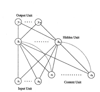
Theoutputsof the hidden unit dependonthe

out-puts ofthe input unit andthe context unit, while

the outputs of the output unit only depends on

the outputs from the hidden unit. More formally,

we define a SRN

as

follows.

$1\mathrm{u}_{\mathrm{i}^{\ovalbox{\tt\small REJECT}\cup \mathrm{t}\mathrm{U}\mathrm{w}}}\iota$

Figure 1: A simple recurrent network

simple _{recurrent networks and Moore machines}

which

are

also finite automata with output. Our

second result is

a

constructionof a simple

recur-rent network which simulates a Moore machine

under

our

assumption. Therefore, these two

con-structionsshow thatthe computationalcapability

ofsimple recurrent networksisequalto that of

fi-niteautomata with output under

our

assumption.

In section 5, we discuss the relationships

be-tween the number of states ofa finite automaton

with output and the size of a simple recurrent networks.

2

Preliminaries

2.1 Simple

Recurrent

Networks

A $S\dot{i}mple$ recurrent network (SRN) consists of

an

$\dot{i}nput$ unit, an output $un\dot{i}t$, a hidden unit and

a

context $un\dot{i}t$ (see Figure 1). The hidden unit, the

context unit and the output unit aresets of gates

each of which computes a function $f[w_{1}, \ldots, w_{m}]$

($x_{1,\ldots,x_{m})}$ : $\mathrm{R}^{m}arrow \mathrm{R},$

$w_{1},$ $\ldots,$$w_{m}\in \mathrm{R},$ $m\in \mathrm{N}$

definedby $f[w_{1}, \ldots,w_{m}](x_{1}, \ldots, x_{m})=\{$ $0$ if _{$\sum_{i=1}^{m}w:xi<0$} $\sum n$ wixi if $0 \leq\sum_{i=1}^{m}w:x:\leq 1$ $:_{=}1$ 1 if $\sum_{1=1}^{m}.w:xi>1$.

For convenience, we $\mathrm{s}\mathrm{h}\mathrm{a}\mathrm{U}$

use

$F$[

$\sum_{i=}^{m_{1}}$ wixi]

in-stead of$f[w_{1}, \ldots, w_{m}](X1, \ldots, xm)$ bom here on.

The context unit ofaSRN holds a copy of the

outputs of the hiddenunitat

a

previoustimestep.

Definition 2.1 A $S\dot{i}mple$ recurrent network is a

7-tuple$\mathcal{E}=(G, I, O, H, C, A, w)$, where

1. $G=(V, E)\dot{i}S$ a directed _{graph, where} $V$

is a

_finite

set

_of

nodes $wh_{\dot{i}C}h$ is divided

into the following

_four

sets

_of

gates: an

in-put $un\dot{i}tI=\{x_{1}, \ldots , x_{n}\}\subseteq V$, an

out-put unit $O=\{y_{1}, \ldots, y_{m}\}\subseteq V$, a hidden

unit $H=\{h_{1}, \ldots, h_{k}\}\subseteq V$ and a

con-text $un\dot{i}tC=\{c_{1}, \ldots, c_{k}\}$ $\subseteq$ V. Then,

$E=\{(v_{1}, v_{2})|(v_{1}, v_{2})\in I\cross H\cup C\cross H\cup H_{\mathrm{X}}$

$C\cup H\cross O\}\dot{i}S$ a set

of

edges

of

G. Edges

from

the $h_{\dot{i}}dden$ unit to the context $un\dot{i}t$ must be

of

the

_form

$(h_{iC_{i}),h_{i}},\in H,$ $c_{i}\in C,$$1\leq\dot{i}\leq k$

.

2. $A=\{A_{1}, \ldots, A_{k}\}\in \mathrm{R}^{k}\dot{i}S$ a set

of

$k$ real

numbers, called $in\dot{i}t\dot{i}al$ output

of

the context

unit.

3. $w$ : $Earrow \mathrm{R}\dot{i}S$ a weight assignment to the

edges $\dot{i}n$ E. We denote the weight

of

an edge

$(v_{1},v_{2})$ by $w(v_{1}, v_{2})$

.

We

assume

that the

weight

_of

the edge $(h_{i,\mathrm{Q}}),$$h_{i}\in H,$ $c_{i}\in C,$$1\leq$

$i\leq k\dot{i}S\mathit{1}$

.

In. this paper,

we

adopt the following realistic

assumption

on

gates ofsimplerecurrent networks:

Assumption 2.1 A $funct\dot{i}on$ computed at each

gate

_of

a simple recurrent network is a $funct\dot{i}on$

whose range is a

_finite

set.

This

means

that we

can

only physically

imple-ment a logic gate whose output is a value of

fi-niteprecision. Rom Assumption1, for each gate,

there exists a finiteset of realnumbers which the

gate

can

output. We define

a

finite ordered set

VALwhichcontainsthese real numbers

as

follows:

VAL $=$

{

$val_{1},$

$\ldots,$$val_{i},$$\ldots$,

valj,

...,$val_{p}$

},

where $val_{k}\in \mathrm{R},$ $1\leq k\leq p,$ $0\leq val_{i}<valj$ $\leq$

$1,\dot{i}<j,\dot{i},j,$$k\in$ N. In the sequel,

we

assume

that a gate compute

a

function $F[ \sum_{i}^{m}=1wiXi]$ :

$\mathrm{R}^{m}arrow \mathrm{V}\mathrm{A}\mathrm{L},$ $m\in \mathrm{N}$

.

Now, we define an input sequence and

an

out-put sequence of

a

SRN. For $v\in V,$$t\geq 0$, let $S_{v}(t)$

denote the output of the gate $v$ at time $t$

.

The

sequence $S_{x_{1}}(t)\cdots s_{x_{n}}(t)$

,

where $x_{i}\in I,$$S_{x_{i}}\in$

$\{0,1\},$ $1\leq\dot{i}\leq n$

.

The output of a SRN at

time $t\geq 2$ isthesequence $S_{y_{1}}(t)\cdot \mathrm{v}\cdot S_{y_{m}}(t)$, where

$y_{i}\in O,$ $1\leq\dot{i}\leq m$

.

Definition 2.2 An input sequence$\mathcal{I}$ with length

$n$ is $\mathcal{I}=\mathcal{I}(0)\mathcal{I}(2)\mathcal{I}(4)\cdots \mathcal{I}(2(n-1))$

.

For

$a$ input sequence $\mathcal{I}$ with length _$n$ and a $SRN$

$\mathcal{E}$, an output sequence

of

$\mathcal{E}$ is $T_{\mathcal{E}}(\mathcal{I})$ _$=$

$\mathcal{O}(2)\mathcal{O}(4)\mathcal{O}(6)\cdots \mathcal{O}(2n)$

.

2.2

Mealy

Machines

A Mealy mach\’ine is a deterministic finite

au-tomaton with output $[1, 6]$

.

Definition 2.3 A Mealy machine$M$ is a 6-tuple

$M=(Q, \Sigma, \Delta, \delta, \lambda, q\mathrm{o})$

,

where $Q$ is a

finite

set

of

states, $q_{0}\in Q$ is

an

initial state, $\Sigma$ is an input

alphabet, $\triangle$ is an output alphabet, $\delta$ : _{$Q\cross\Sigmaarrow Q$}

is a transitionfunction, and $\lambda$ : _{$Q\cross\Sigmaarrow\Delta$} is an

output

_function.

Let $q(t)\in Q$ denote the state of $M$ at time

$t$

.

We define

an

input sequence and an output

sequence ofa Mealy Machine

as

follows:

Definition 2.4 An input sequence $w$

of

a Mealy

machine with length $i\in \mathrm{N}$, is a string _$w=$

$a_{0}a_{1}\cdots a_{i-1},$ $a_{j}\in\Sigma,$ $0\leq j\leq i-1$

.

Definition 2.5 For an input sequence $w$ $=$

$a0a_{1}\cdots ai-1$, an output sequence

of

a Mealy

ma-chine $M,$ $T_{M}(w)$ is a string

$T_{M}(w)=\lambda(q(\mathrm{O}), a\mathrm{o})\lambda(q(1), a_{1})\cdots\lambda(q(\dot{i}-1), ai-1)$

such that$q(t+1)=\delta$($q(t)$,at), $0\leq t\leq\dot{i}-1$

.

We define an equivalence relation between simple

recurrent machines and Mealy machines.

Definition 2.6 A $SRN\mathcal{E}$ is said to be equivalent

to a Mealy machine $M$

if

$T_{\mathcal{E}}(W)=T_{M}(w)$

for

any $\dot{i}nput$sequence $w$

.

2.3

Moore

Machines

$.\mathrm{A}$ Moore machine is also a deterministic finite

automaton with output [6].

Definition 2.7 A Moore machine$M$ is a 6-tuple

$M=(Q, \Sigma, \Delta, \delta, \lambda, q\mathrm{o})$, where $Q$ is a

finite

set

of

states, $q_{0}\in Q$ is an initial state, $\Sigma$ is

an

input alphabet, $\Delta$ is an output alphabet, $\delta$: _{$Q\cross\Sigmaarrow Q$}

is a transition function, and $\lambda$ : _{$Qarrow\triangle$} is an

output

_function.

We define

an

input $\grave{s}equence$and

an

output

se-quence of

a

Moore machine in the

same

fashion of

those of

a

Mealy machine. The following lemma

is known [6].

Lemma 2.1 For

a

Mealy machine $M’$, there

ex-ists a Moore machine $M$ which is equivalent to

$M’$

.

2.4

Vector representations

Suppose that the number ofstates of a Moore

machine $M=(Q, \Sigma, \Delta, \delta, \lambda, q\mathrm{o})$ is $m$

,

the

num-ber of elements of the input alphabet is $k$

,

and

the number of elements of the output alphabet

is $l$

.

Namely, let $Q=\{q_{0}, \ldots, q_{m}-1\},$ $\Sigma=$

$\{a_{0}, \ldots, a_{k}-1\}$ and $\Delta=\{b_{0}, \ldots, b_{l-}1\}$

.

We first define

a

state vector of

a

Moore

ma-chine. Each entry of a state vector corresponds

to a tuple of

a

state and an input symbol of a

Moore machine.

Definition 2.8 A state vector

_of

$M$ at time $t$ is

$v(t)\in\{0,1\}^{km}$ and

satisfies

thefollowing

proper-ties:

1.

_If

$t=0$ _and$q(t)=q_{i}$,

from

the$\dot{i}k+1$th entry

to the $\dot{i}k+kth$ entry

of

$v(t)$

are

all l’s and

the others are $0^{)}s$

.

2.

_If

$t\neq 0$ and $q(t)=q_{i}$, only one entry

from

the$ik+1$th entry to the$\dot{i}k+kth$ entry

of

$v(t)$

is 1 and the others are $\mathrm{O}’ s$

.

Next,

we

define

an

input vector of

a

Moore

ma-chine. Let $I(t)$ denote

a

given input symbol ofa

Moore machine at time $t$

.

Definition 2.9 An input vector

_of

$M$ at time $t$

is $w(t)\in\{0,1\}^{k}$, and

if

$I(t)=a_{i}$, the $i+1$th

entry

_of

$w(t)$ is 1 and the others are $\mathrm{O}’ s$

.

We define

a

state-input vector based onthe above

definitions.

Definition 2.10 Let$v(t)=(v_{1}(t), \ldots, vkm(t))\in$

$\{0,1\}^{km}$ a state vector and $w(t)=(w_{1}(t),$ $\ldots$, $w_{k}(t))\in\{0,1\}^{k}$ an input vector

of

$M$ at time

$t$

.

Then, a state-input vector

of

$M$ at time $t$

is $V(t)=(v_{1}(t), \ldots, vkm(t), w_{1}(t), \ldots, wk(t))\in$

$\{0,1\}^{km}+k$

.

Next, we define an output vectorof a Moore

ma-chine. Let $O(t)$ denote an output symbol of a

Definition 2.11

_If

an output vector $\cdot ofM$ at

time $t\dot{i}su(t)\in\{0,1\}^{l}$, and $O(t)=b_{i}$, then the

$i+1$th entry

of

$u(t)$ is 1 and the others are $\mathrm{O}’ s$

.

Finally, we give the definition of equivalence

relation between simple recurrent networks and Moore machines.

Definition 2.12 For $a$ input sequence _{$w,$ $\sup-$}

pose that a Moore machine $M$ yeilds the output

sequence $T_{M}(w)$ and a $SRN\mathcal{E}$ yeilds the output

sequence $T_{\mathcal{E}}(w)$

.

Then, $\mathcal{E}$ is _$sa\dot{i}d$ to be equivalent

to $M$

if

_{$T_{M}(w)=bTg(w)$}

for

all_$w$ where $b$ is the

output alphabet

_for

the initial state

_of

$M$.

3

Constructing

Mealy

Mach-ines

In this section, we will construct a Mealy

ma-chine which isequivalent to

a

given SRN. We

de-scribe how to define thestates,thetransition

func-tionand the output functionofthe SRN.

Suppose that aSRN$\mathcal{E}=(G, I, O, H, C, A, w)$ is

given, where $|I|=n,$$|O|=m,$ _$|H|=|C|=k$

.

We

construct aMealy machine$M=(Q, \Sigma, \Gamma, \delta, \lambda, q_{0})$

which simulates $\mathcal{E}$ in the following way.

1. Each state$p\in Q$ of$M$ represents the output

pattern $a_{c_{1}}\cdots a_{c_{k}}$ of the context unit, where $a_{c_{t}}\in$ VAL and $\mathrm{q}\in C$

.

Note that every

out-put pattern of the context unit

can

be

repre-sented as a word in VAL$k$

.

Thus, the states

of $M$ includes all the repreS.entation of the

output pattern of the context unit of$\mathcal{E}$

.

The initial output pattern of the context unit of$\mathcal{E}$

corresponds to the initial state$$q0$ of$M$

.

2. Since the number of the gates in the context

unit is equal to that of the hidden unit, each

state $p\in Q$ of $M$ also represents the output

pattern $a_{h_{1}}\cdots a_{h_{k}}$ of the hidden unit, where

$a_{h_{\mathfrak{i}}}\in \mathrm{V}\mathrm{A}\mathrm{L}$ and $h_{i}\in \mathcal{H}$

.

for each $i,$ $1\leq i\leq k$

.

Then, the transition

function $\delta$ of $M$ is defined

by $\delta(p, \sigma)=p’$

where $p=a_{c_{1}}\cdots a_{c_{k}}\in Q,$$\sigma=a_{x_{1}}\cdots a_{x_{n}}\in$ $\Sigma$ and $p’=a_{h_{1}}\cdots ah_{k}\in Q\mathrm{S}\mathrm{a}\mathrm{t}\mathrm{i}\mathrm{s}\mathfrak{g}\Gamma$the above

equations.

4. Finally, we construct the output function $\lambda$

of $M$

.

Suppose that the output pattern of

the input unit of $\mathcal{E}$ is

$a_{x_{1}}\cdots a_{x_{n}}$, the

out-put pattern of the context unit is $a_{c_{1}}\cdots a_{c_{n}}$

and the output pattern of the hidden unit is

$a_{h_{1}}\cdots a_{h_{k}}$

.

The output of$\mathcal{E}$ depends on the

output pattern of the hidden unit. That is,

the output of the gates$a_{y_{i}}$ inthe output unit

is given by

$a_{yi}=F[ \sum_{j=1}^{k}w(h_{j,y_{i})]}ah_{k}$

.

Then, the output function $\lambda$ of$M$ is defined

by $\lambda(p, \sigma)=\gamma$where _{$p=a_{c_{1}}\cdots a_{c_{k}}\in Q,$}$\sigma=$ $a_{x_{1}}\cdots a_{x_{n}}\in\Sigma,$ $\gamma=a_{y_{1}}\cdots a_{y_{m}}\in Q\mathrm{s}\mathrm{a}\mathrm{t}\mathrm{i}\mathrm{S}\mathfrak{h}\Gamma$

the above equations. We have the following result:

Theorem 3.1 Under Assumption 2.1,

_for

any

simple recurrent network$\mathcal{E}$, there exists a Mealy

machine $M$ which is equivalent to $\mathcal{E}$

.

4

Constructing

Simple

Recur-rent

Networks

In this section, we will show that there exits

a

SRN which simulates a Moore Machine. For this

purpose, we

use

a connection matrix of a Moore

machine [2]. Our first goal is to show that

a

con-nection matrix ofa Moore machine

can

be

imple-mented

on

a

SRN. Throughthissection, consider

a

Moore machine$M=(Q, \Sigma, \Delta, \delta, \lambda, q\mathrm{o})$with$Q=$ $\{q_{0}, q_{1}, \ldots, qm-1\}$ and $\Sigma=\{a0, a_{1}, \ldots, ak-1\}$

.

3. We construct the transitionfunction $\delta$ of$M$

.

Suppose that the outputpatternof the input

unit of$\mathcal{E}$ is

$a_{x_{1}}\cdots a_{x_{n}}$ and the output pattern

of the context unit of $\mathcal{E}$ is

$a_{c_{1}}\cdots a_{\mathrm{c}_{n}}$

.

The

output pattern of the hiddenunitdependson

$a_{c_{1}}\cdot*\cdot ac_{k}$ and$a_{x_{1}}\cdots a_{x_{n}}$

.

That is, the output

of the gate $a_{h_{f}}$ in the hidden unit is given by

$a_{h_{i}}=F[_{j=1} \sum^{k}w(Cj, h_{i})a_{c}j+\sum_{j=1}^{n}w(Xj, h_{i})axj]$ ,

4.1

Connection matrices

Wefirst define a connection matrix ofa

transi-tion functransi-tion ofa Moore machine [2].

Definition 4.1 A connection matrix $\alpha$

of

transi-tion

_function

_of

$M$ is

$\alpha_{ij}=\{x\in\Sigma|\exists q_{iq_{j}},\in Q, \delta(q_{i}, x)=qj\}$,

where $\alpha_{ij}$ is an entry

of

the $\dot{i}th$ row and the $jth$

4.2

Weight

matrices

From the definition, a connection matrix $\alpha$ of

$M$isan$m\cross m$matrix. We define a weight matrix

$\mathrm{o}\mathrm{f}M$

.

Definition 4.2 For a Moore machine $M$, $a$

weight matrix$\alpha’$

of

_$M$ is a $km\cross(km+k)$ matrix

which

_satisfies

the following properties:

$\bullet F_{or}\dot{i}ifand’ Oj,nly\dot{i}fihereex’,0\leq 1\leq\dot{i},j\leq km_{istSh}iheen\iota ry\alpha_{ij}’\dot{i}S\frac{1}{-1,k+1}h\leq k$

such that $\delta(q_{\lfloor}(i-1)/k\rfloor’ ah)=q_{\lfloor}(j-1)/k\rfloor$ _’ and

the entry $\alpha_{ij}’$ is $0$

if

and only

if

there does

not exist $h,$ $0\leq h\leq k-1$, such that

$\delta(q_{\lfloor}(i-1)/k\rfloor’ ah)=q\lfloor(j-1)/k\rfloor$

.

.

For$\dot{i},j,$ $1\leq\dot{i}<km$, $km\leq j\leq km+k$, the

entry$\alpha_{ij}’$ is $\frac{2k+\overline{1}}{2k+2}$

if

(j-km) mod $k=\dot{i}$ mod$k$

and the entry $\alpha_{ij}’$ is

$\mathit{0}$

if

(j–km) mod $k\neq$

$\dot{i}$ mod$k$

.

Now, weconstruct aweight matrix$\alpha’\mathrm{h}_{\mathrm{o}\mathrm{m}}$a

con-nection matrix $\alpha$ as follows:

SRN is a finite set, namely VAL$=\{0,1\}$

.

There-fore,

a

function computed at each gate is

$F[ \sum_{i=1}^{m}wi^{X]}i=\{$

$0$ if $\sum_{i=1}^{m}$$wixi<0$ $0$ if $0 \leq\sum_{i=1}^{m}$$wixi\leq 1$

1 if $\sum_{i=1}^{m}$$wixi>1$

.

We will define a function $\sigma$ from the function$F$

.

Definition 4.3 For an $n\cross m$ matrix$A$, a

func-tion $\sigma_{A}$

:

$\{0,1\}^{m}arrow\{0,1\}^{n}$ is

$\sigma_{A}(x)=$

,

where $x=$ $(x_{1}, \ldots , x_{m})$ and

$A=$

.

1. Let $\alpha^{T}$ be atransposed matrix of $\alpha$

.

2. For an$m\cross m$ matrix$\alpha$ of$M$, let a matrix $\alpha’$

be a $km\cross(km+k)$ matrix.

3. Entries in the 1st,...,the kmth rows and the

1st,..., the kmth columns of $\alpha’$

are

defined

as:

(a) If the entry $\alpha_{ij}$ contains a symbol $at\in$

$\Sigma,$ $k$ entries in the $k(j-1)+1\mathrm{t}\mathrm{h},$ $\ldots$,

the$k(j-1)+k\mathrm{t}\mathrm{h}$columns and the $k(\dot{i}$ -$1)+t\mathrm{t}\mathrm{h}$

row

are all $\frac{1}{k+1}$

.

(b) If the entry$\alpha_{ij}$ does notcontains a

sym-bol$at\in\Sigma,$ $k$entriesin the$k(j-1)+1\mathrm{t}\mathrm{h}$,

...,

the $k(j-1)+k\mathrm{t}\mathrm{h}$ columns and the

$k(\dot{i}-1)+t\mathrm{t}\mathrm{h}$row are all$0$

.

4. Entries in the 1st, ...,thekmthrows and the

$km+1\mathrm{t}\mathrm{h},$ $\ldots$, the$km+k\mathrm{t}\mathrm{h}$columns of

$\alpha’$ are

defined

as

follows: for the$\dot{i}\mathrm{t}\mathrm{h}$row, anentry in

the ith

row

andthe $km+$($i$mod $k$)$\mathrm{t}\mathrm{h}$column

of$\alpha’$ is

$\frac{2k+1}{2k+2}$ and the other entries

are

all $0$

.

4.3

Implementing

matrices on

simple

recurrent networks

In thispaper,

we

already have

assume

that the

range of a function computed at each gate of

a

The outputs of units of SRN’s

are

regarded as

vectors. A transition functionof$M$

can

be

imple-mented by using a function $\sigma_{\alpha’}$

.

Lemma 4.1 Suppose that $\delta(q_{i}, a_{j})=q_{h}$, a state

vector

_of

the state $q_{i}$ is $v$

, an

input vector

of

the

input symbol $a_{j}$ is $w$, and a state-input vector

of

$v$ and $w$ is V. Then, a vector $\sigma_{\alpha’}(V)$ is a state

vector

_of

the state $q_{h}$

.

4.4

Constructing

simple

recurrent

net-works which simulate Moore

ma-chine.

$\mathrm{s}$

In thissection,

we

willconstruct

a

SRNwhich is

equivalenttoagiven Moore machine. Wedescribe

howtodefine the input unit, the output unit, the

context unit, the hidden unit, the initial output and the weights.

Let$M=(Q, \Sigma, \Delta, \delta, \lambda, q\mathrm{o})$ be

a

Moore machine . _{and $m=|Q|,$} $k=|\Sigma|$, and $l=|\Delta|$

.

We will

con-struct

a

SRN $\mathcal{E}=(G, I, O, H, C, A, w)$

as

follows:

1. The input unit is $I=\{x_{1}, \ldots, x_{k}\}$

.

2. The output unit is $O=\{y_{1}, \ldots, y\iota\}$

.

3. The context unit is $C=\{c_{1}, \ldots, C_{k}m\}$, and

4. Let $v(\mathrm{O})$ be a state vector of the initial state $q_{0}$ and $v(\mathrm{O})=(v_{1}(0), \ldots, vkm(0))$, where

$v_{i}(0)\in\{0,1\},$$1\leq\dot{i}\leq km.$ Then, the

ini-tialoutput$A$is _{$A=\{A_{1}, A_{2}, \ldots A_{km}\}$}, where

$A_{i}=v_{i}(\mathrm{O}),$ $1\leq i\leq km$.

5. Note that $t$he weight matrix $\alpha’$ of _$M$ is a

$km\cross(km+k)$ matrix. We definethe weights

as follows:

(a) Foranedge $(x_{i}, h_{j}),$$xi\in I,$ $h_{j}\in H$, the

weight $w(X_{i}, h_{j})$ is the entry in the $j\mathrm{t}\mathrm{h}$

row and $km+1t\mathrm{h}$ column of$\alpha’$

.

(b) For a edge $(c_{i}, h_{j}),$ $c_{i}\in C,$ $h_{j}\in H$, the

weight $w(C_{i}, h_{j})$ is the entry in the $j\mathrm{t}\mathrm{h}$

row

and $\dot{i}\mathrm{t}\mathrm{h}$ column $\mathrm{f}\alpha’$

.

6. If $\lambda(q_{i})=b_{j}$, the weight $w(h_{s}, y_{j})$ is an

ar-bitrary value that is greater than 1 for $h_{s}$,

$\dot{i}k\leq s\leq\dot{i}k+k$. The weights of the other

edges are all $0$

.

We obtain the following theorem.

Theorem 4.1 Under Assumption 2.1,

_for

any

Moore machine $M$, there exists a simple

recur-rent network$\mathcal{E}_{M}$ which is equivalent to $M$

.

5

The

Size

of Simple

Recurrent

Networks

In this section, wediscuss the relationships

be-tween the number ofstates ofautomatawith

out-put and the size of a SRN. Suppose that a SRN

$\mathcal{E}$ is equivalnet to automata with output $M$

.

Let

$K(M)$ be a set ofautomata which

are

_equivalnet

to $M$and$S(\mathcal{E})$ be aset of SRN’s which

are

equiv-alnet to $\mathcal{E}$

.

For $M$, let

$\phi(M)$ denote

a

number of

the states of $M$

.

For $\mathcal{E}$, let

$S\dot{i}Ze(\mathcal{E})$ denote the

size of$\mathcal{E}$, where the size of

a

SRN is

the number of gates of$\mathcal{E}$

.

Definition 5.1 $M_{\min}$ is $a$ element

of

$K(M)$

w.hich

satisfies

$\phi(M_{\min})=\min\{\phi(M)|M\in K(M)\}$

.

Definition 5.2 $\mathcal{E}_{\min}$ is $a$ element

of

$S(\mathcal{E})$ which

satisfies

$S \dot{i}ze(\mathcal{E}_{\min})=\min\{size(\mathcal{E})|\mathcal{E}\in S(\mathcal{E})\}$

.

From the above two construction, we obtain the

following theorem.

Theorem 5.1 For$M$ and$\mathcal{E}$, there exit constants

$C$ and $C’$ such that

6

Conclusion

In this paper, we show that when the range of

a function computed at each gate of

a

SRN is

a finite set, there exists

a

Mealy machine which

can

simulates the SRN. This result

means

that,

under

our

assumption, the computational power

of simple recurrent networks is not exceed $t$hat

offinite automata with output, and thus, is not

sufficient to recognize natural languages.

On the other hand, asimple recurrent network

can simulates a Moore machine as we showed in

Section4.4. From

our

two results, wehave shown

that the computationalcapabilityofsimple

recur-rent networks is equal to that offinite automata

under our assumption.

References

[1] Noga Alon, A. K. Dewdney, and Teunis J. Ott.

Ef-ficient simulation of finite automata by neural nets.

Joumal_{ofAssociaiionfor}Computing Machinery, Vol. 38, No. 2, pp. 495-514, April 1991.

[2] M. A. Arbib, A. J. Kfoury, and Robert N. Moll. $A$

Basis _for Theoretical Computer Science. Springer-Verlag, 1981.

[3] Jose’ L. Balca’zar, Ricard Gavald\‘a, Have T. Siegel-mann, and Eduardo D. Sontag. Somestructural

com-$\mathrm{p}\mathrm{l}\mathrm{e}\mathrm{x}\mathrm{i}\mathrm{t}\dot{\mathrm{y}}$aspects of neural computation. In Proceedings

ofthe IEEEStructure in Complexity Theory Confer-ence, pp. 253-265, San Diego, CA, 1993.

[4] $\mathrm{J}\mathrm{e}\mathrm{f}\mathrm{f}\mathrm{r}_{le}\mathrm{e}\mathrm{L}.\mathrm{E}tivecienC1,\mathrm{m}\mathrm{a}n.\cdot \mathrm{F}\mathrm{i}\mathrm{v}_{0}1\mathrm{l}4,\mathrm{p}\mathrm{p}.1\mathrm{n}\mathrm{d}\mathrm{i}\mathrm{n}\mathrm{g}\mathrm{s}\mathrm{t}\mathrm{r}\mathrm{u}_{21}\mathrm{C}\mathrm{t}\mathrm{u}\mathrm{r}\mathrm{e}\mathrm{i}\mathrm{n}079-1,199.\mathrm{i}\mathrm{t}\mathrm{m}\mathrm{e}$

.

Congni-[5] JeffreyL. Elman. Distributed representations, simple recurrent networks and grammatical structure.

Ma-chineLearning,

Vol.

7, pp. 195-225, 1991.

[6] J. E. Hopcroft and J. D. Ullman. Introduction to Au-tomata Theory, Language and Computation. Read-ing. Addison-Wesley, MA, 1979.

[7] P. Indyk. Optimal simulation of automata by neural

$\mathrm{n}\mathrm{e}\mathrm{t}\mathrm{S}.\mathrm{I}\mathrm{n}\tau heoreiCa\iota^{r_{Atso}}Pocespecfedin\mathit{9}^{so}fhe\mathit{1}\mathit{2}thAnnualSym_{\oint g^{on}}osimc^{t}omputersCience(SAc^{u}s’ \mathit{5})$ ,

pp. 337-348, New York, April 1995. Springer-Verlag. [8] James L. $\mathrm{M}\mathrm{c}\mathrm{C}\mathrm{l}\mathrm{e}\mathrm{n}_{\mathrm{a}\mathrm{n}}\mathrm{d}$, Axel Cleeremans, and David

Servan-Schreiber. Paralleldistributedprocessing:

Br-idging the gap between human and machine

mtelli-gence. Joumal_ofJapanese Society_ofArtificial Intel-ligence, Vol. 5, No. 1, pp. 3-14, January 1990. [9] 守谷純之介, 西野哲朗. 「単純回帰ネットワークを模倣

するmealy機械の構成法」

.

電子情報通信学会コンピュ

テーション研究会資料. COMP98-27. 1998.

[10] Have T. Siegelmann and Eduardo D. Sontag. On the

$\mathrm{c}\circ \mathrm{m}the\mathrm{F}^{\mathrm{u}}iflhA^{\circ}cMWorksh_{\mathit{0}}p_{\mathit{0}}nComputationa\iota^{ee}Lea\mathrm{r}nin^{O}g\mathrm{t}\mathrm{a}\mathrm{t}\mathrm{i}\mathrm{n}\mathrm{a}\mathrm{l}\mathrm{P}^{\mathrm{O}}\mathrm{w}\mathrm{e}\mathrm{r}\mathrm{o}\mathrm{f}\mathrm{n}\mathrm{e}\mathrm{u}x\mathrm{a}1\mathrm{n}\mathrm{e}\mathrm{t}\mathrm{S}.\ln ProCding_{S}f$

Theory, Pittsburgh, PA, July1992.

[11] Have T. Siegelmann and Eduardo D. Sontag. Analog computation via neural networks. Theoretical

Com-puterScience, Vol. 131,pp. 331-360, 1994.