Three-dimensional instability of Kirchhoff's elliptic vortex : Its relation to the elliptical instability(Mathematical Fluid Mechanics and Modeling)

Three-dimensional instability of Kirchhoffl$s$

elliptic vortex

- Its relation to the elliptical instability

-Univ. Electro-Communications Takeshi Miyazaki ( $\hat{@}$;li

ffi

) Nagoya Univ. Yasuhide Fukumoto $( \dagger^{H}\mathbb{R}*\ovalbox{\tt\small REJECT} \mathfrak{F} )$

1.

Introduction

The three-dimensional instability modes of concentrated

vortices

are

classified into two categories according to their axial

wavelengths. One with the longer wavelength (much longer than

the vortex

core

radius) is called the Crow instabilit$y^{}$ , which

explains the destabilization of trailing vortices shed from

an

aircraft. Tsai

&

Widnall2

and Moore

& Saffman3

found that

a

columnar vortex embedded in a strain field is unstable to the

bending perturbations whose axial wavelength is order of the

core

radius. Widnall, Bliss

&

Tsai4

succeeded in explaining the destabilization of

a

vortex ring following the

same

lines of consideration.

Recently,

Pierrehumbert5

showed numerically that

an

unbounded inviscid strained vortex undergoes instability whose

growth rate is independent of wavelength.

Bayly6

formulated the problem

as

a

matrix Floquet problem, which suggested that the instability is prametrically excited. It is, by now, _{recognized that}

the Floquet-mechanism is the

essence

of the short-wave instabilities.

Waleffe7

gave,

in the limiting

case

of weak strain,

a

clear physical explanation of the instability

as

a

resonant

interaction between the inertial

wave

and the imposed strain field. These instabilities

are

called the elliptical instability, since

they

are

induced whenever streamlines of

a

basic flow endowed with vorticity

are

deformed elliptically. It is not difficult to

incorporate the viscous effect, which

was

undertaken by Landman

and

Saffman8.

They showed that this intrinsically inviscid

instability mechanism persists

even

in the presence of the viscous

dissipation.

Craik9

proposed to incorporate the contribution of various types of body force and described the influence of

a

question of the effect of

a

buoyancy force and

Miyazakil

1

considered the combined effect of both forces

on

the elliptical

instability.

In spite of the abundance of studies

on

the elliptical instability, the relevance of the mechanism to the actual flow fields is not

fully understood. Gledzer and

Ponomarev12

investigated the

instability of

a

solid body rotation of fluid in

an

elliptical cylinder

and compared their results with the predictions of the elliptical instability. The numerical

investigations13-15

of Poiseuille flows have revealed that finite-amplitude two-dimensional

waves

are

unstable to short-wave three-dimensional instabilities. It is

considered that the continuous instabilities

are

discritized to form

an

infinite number of separate short-wave instability bands, if

an

appropriate outer boundary condition is taken into

account16.

Our objective in this paper is to manifest the broad generality of

the elliptical instability by investigating numerically the linear instability of

an

elliptic vortex patch of finite extent.

Pierrehumbert

&

Widnalll7

investigated the linear stability of the Stuart vortex and Robinson

&

Saffmanl8

considered the Moore-Saffman

vortex19,

before the birth of the concept of elliptical instability. Our work will

serve

to complement these precursors.

Specifically,

we

focus

our

attention

on

Kirchhoffs elliptic

vortex, a vortex patch with uniform vorticity $\omega 0$ inside of

an

ellipse whose major and minor semi-axes

are a

and $b$

.

If it is

embedded in

an

irrotational fluid, it rotates solidly with

a

constant

angular velocity $\Omega=\omega 0ab/(a+b)^{2}$

.

A century ago, $Love2$ studied the

two-dimensional linear instability of the Kirchhoffs elliptic vortex

and found that it becomes unstable to disturbances with azimuthal

wave

number 3, if the ratio $a/b$ is greater than 3. As for

the three-dimensional stability, Vladimirov

&

Il$\prime in^{21}$ made

an

asymptotic analysis in the limit of small eccentricity, and showed

that there

are

infinite number of instability

bands.

Our numerical

analysis extends their results to the

case

of finite ellipticity.

2. Formulation

Let

us assume

that the fluid is inviscid and incompressible. The

streamfunction (in the inertial frame) inside of Kirchhoffs elliptic

vortex is given $by^{20}$,

$\Psi_{in}^{(i)}=-\frac{bx^{2}+ay^{2}}{2(a+b)}$ , (1)

where the uniform vorticity $\omega 0$ in the interior of the ellipse is

taken to be unity and $a$ is the major semi-axis and $b$ is the minor

semi-axis. The elliptic vortex rotates rigidly about the z-axis with

a constant angular velocity

$\Omega=\frac{ab}{(a+b)^{2}}$

.

(2)

Hence, the ellipse is stationary if

we

move

into the coordinate

frame rotating with the angular velocity $\Omega$ around the z-axis. The

(rotating) Cartesian coordinates $(x, y, z)$

are

used, hereafter, with

the corresponding unit vectors $e_{x},$ $e_{y}$ and $e_{z}$

.

The streamfunction

(1) in the inertial frame is augmented by

a

collection term as,

$\Psi_{in}=-\frac{bx^{2}+ay^{2}}{2(a+b)}+\frac{1}{2}\Omega(x^{2}+y^{2})$

.

(1’)

It is noted that the interior vorticity is reduced to

$\omega’0=(a^{2}+b^{2})/(a+b)^{2}$ in the rotating coordinates. The

use

of the

elliptic-cylinder coordinates $(\xi, \eta, z)$ is convenient in describing

the geometry of the basic flow field:

$x=$ ccosh$\xi\cos\eta$ , (3a)

$y=$ csinh$\xi\sin\eta$ , $0\leq\eta\leq 2\pi$, (3b)

where $c=\sqrt{a^{2}- b^{2}}$

and $h^{2}$ denotes the metric factor:

$h^{2}=\frac{1}{2}c^{2}(\cosh 2\xi-\cos 2\eta)$

.

(3c)

In these coordinates, the boundary of the ellipse is represented by

$\xi=\xi_{0}=\frac{1}{2}\log(\begin{array}{l}\omega+a- b\end{array})$, (4)

and the streamfunction outside of the vortex is written

as

$\Psi_{out}=-\frac{ab}{2}\xi-\frac{ab}{4}e^{-2\xi}\cos 2\eta+\frac{1}{2}\Omega(x^{2}+y^{2})$

.

(5)

2.2 Perturbation equations

Since the basic flow is uniform in the z-direction,

we

can

introduce the normal-mode disturbances of small amplitude with the form proportional to $e^{i(kz-\omega t)}$_, where _$k$ is the axial wavenumber:

$u\dot{\xi}^{n}=U\dot{\xi}^{n}+\overline{\epsilon}u\xi e^{i(kz-\omega t)}$, $u_{\eta}^{in}=U_{\eta}^{in}+\overline{\epsilon}u_{\eta}e^{i(kz- t0t)}$,

(6) $w^{in}=\overline{\epsilon}\overline{w}e^{i(kz-\omega t)}$,

$p^{in}=P^{in}+\overline{\epsilon}\overline{p}e^{i(kz- 0)t)}$, where $\overline{\epsilon}$ is

a

small

parameter $(\overline{\epsilon}<<1)$

.

Since the flow is irrotational

outside of the ellipse,

we

may

assume

that the disturbances

are

irrotational, too, there:

$u\not\in u\iota_{=U_{\xi^{ut}}^{O}+\overline{\epsilon}\frac{\partial\overline{\phi}}{h\underline{\partial\xi}}e^{i(kz- t0t)}}$ ,

$u_{\eta}^{out}=U_{\eta}^{out}+\overline{\epsilon}\frac{\partial\phi}{h\partial\eta}e^{i(kz-\omega t)}$, (7)

$w^{out}=W^{out}+\overline{\epsilon}ik\phi e^{i(kz-\omega t)}$

.

The linearized Eulerian equations of motion in the elliptic-cylinder coordinates

are

$- i\mathfrak{c}0\overline{u}+\frac{1}{h^{2}}[\overline{U}\frac{\partial}{\partial\xi}+\overline{V}\frac{\partial}{\partial\eta}]\overline{u}+\perp h^{2}[\overline{u}\frac{\partial}{\partial\xi}+\overline{v}\frac{\partial}{\partial\eta}]\overline{U}$ (8a) $+( \overline{U}\overline{u}+\overline{v}v\gamma\frac{\partial}{\partial\xi}(\frac{1}{h^{2}})- 2\Omega\overline{v}=-\frac{\partial\overline{p}}{\partial\xi}$ $- i\omega\overline{v}+\frac{1}{h^{2}}[\overline{U}\frac{\partial}{\partial\xi}+\overline{V}\frac{\partial}{\partial\eta}]\overline{v}+\frac{1}{h^{2}}[\overline{u}\frac{\partial}{\partial\xi}+\overline{v}\frac{\partial}{\partial\eta}]\overline{V}$ (8b) $+( \overline{U}\overline{u}+\overline{V}\overline{v})\frac{\partial}{\partial\eta}(\frac{1}{h^{2}})+2\Omega\overline{u}=-\frac{\partial\overline{p}}{\partial\eta}$

-i

$(0 \overline{w}+\frac{1}{h^{2}}[\overline{U}\frac{\partial}{\partial\xi}+\overline{V}\frac{\partial}{\partial\eta}]\overline{w}=- ik\overline{p},$ (8c) $\perp h^{2}(\frac{\partial\overline{u}}{\partial\xi}+\frac{\partial\overline{v}}{\partial\eta})+ik\overline{w}=0$, (9)

where

new

dependent variables $\overline{u}=hu\xi$ and $\overline{v}=hu_{\eta}$ with $\overline{U}=hU\dot{\xi}^{n}$

and $\overline{V}=hV\dot{\xi}^{n}$

are

introduced. Note that the Coriolis terms

proportional to $2\Omega$

are

added to those given by Robinson

&

Saffman18.

Eliminating $\overline{w}$

and $\overline{p}$ using the continuity equation (9)

and the third component of the Eulereian equation (8c),

we are

left with coupled equations for $\overline{u}$ and $\overline{v}$

:

$- i\omega\{\overline{u}_{k^{2}}-\perp\frac{\partial}{\partial\xi}[\frac{1}{h^{2}}(\frac{\partial\overline{u}}{\partial\xi}+\frac{\partial\overline{v}}{\partial\eta})]\}=-\frac{1}{h^{2}}(\overline{U}\frac{\partial}{\partial\xi}+\overline{V}\frac{\partial}{\partial\eta})\overline{u}- h^{2}\perp cu\frac{\partial}{\partial\xi}+\overline{v}\frac{\partial}{\partial\eta})\overline{U}$

$-( \overline{U}\overline{u}+\overline{V}_{V}\circ\frac{\partial}{\partial\xi}(\frac{1}{h^{2}})+2\Omega\overline{v}+\frac{1}{k^{2}}\frac{\partial}{\partial\xi}t\frac{1}{h^{2}}(\overline{U}\frac{\partial}{\partial\xi}+\overline{V}\frac{\partial}{\partial\eta})[\frac{1}{h^{2}}(\frac{\partial\overline{u}}{\partial\xi}+\frac{\partial\overline{v}}{\partial\eta})]\}$

$- i\omega\{\overline{v}-\frac{1}{k^{2}}\frac{\partial}{\partial\eta}[\frac{1}{h^{2}}(\frac{\partial\overline{u}}{\partial\xi}+\frac{\partial\overline{v}}{\partial\eta})]\}=-\frac{1}{h^{2}}(\overline{U}\frac{\partial}{\partial\xi}+\overline{V}\frac{\partial}{\partial\eta})\overline{v}-\frac{1}{h^{2}}Cu\frac{\partial}{\partial\xi}+\overline{v}\frac{\partial}{\partial\eta})\overline{V}$

$-( \overline{U}\overline{u}+\overline{v}v3\frac{\partial}{\partial\eta}(\frac{1}{h^{2}})- 2\Omega\overline{u}+\frac{1}{k^{2}}\frac{\partial}{\partial\eta}\{\frac{1}{h^{2}}(\overline{U}\frac{\partial}{\partial\xi}+\overline{V}\frac{\partial}{\partial\eta})[\frac{1}{h^{2}}(\frac{\partial\overline{u}}{\partial\xi}+\frac{\partial\overline{v}}{\partial\eta})]\}$

$(10a_{2}b)$

Since these equations $(10a,b)$

are

singular at $h=0$, they

are

multiplied by

h@

in implementing the numerical procedure below. The potential $\overline{\phi}(\xi, \eta)$ outside of the vortex obeys the Helmholtz equation:

$[ \frac{\partial^{2}}{\partial\xi^{2}}+\frac{\partial^{2}}{\partial\eta^{2}}- 2q(\cosh 2\xi-\cos 2\eta)]\overline{\phi}=0$, (11)

with $q=\frac{1}{4}c^{2}k^{2}$

.

Equation (11) is separable and the solution is obtainable in the form of expansions in terms of the Mathieu functions.

The boundary of the vortex patch is assumed to deform

as

$\xi=\xi_{0}+\overline{\epsilon}F(\eta)e^{i(kz-\omega t)}$

(12)

At $O(\overline{\epsilon})$, the kinematical boundary conditions that the boundary of

the vortex patch continues to be the boundary

are

written,

on

$\xi=\xi_{0}$,

as

$itoh^{2}F+\overline{u}-\Omega\frac{\partial}{\partial\eta}(h^{2}F)=0$ , (13a)

$i\omega h^{2}F+\frac{\partial\overline{\phi}}{\partial\xi}-\Omega\frac{\partial}{\partial\eta}(h^{2}F)=0$

.

(13b)

The dynamical conditions

on

$\xi=\xi_{0}$ require the continuity of tangential velocity components, which

are

equivalent to the condition of pressure continuity:

$\frac{\partial\overline{\phi}}{\partial\eta}-\overline{v}=h^{2}F$, (14a)

$\frac{\partial^{2}\overline{\phi}}{\partial\xi^{2}}-\frac{\partial\overline{u}}{\partial\xi}=-\frac{\partial}{\partial\eta}(h^{2}F)$

.

(14b)

.

Since the formulation of numerical eigenvalue problems is

essentially identical to those of Robinson

&

Saffman18,

we

will

give only

a

brief outline. The velocity components $\overline{u}$ and $\overline{v}$ inside

of the vortex

are

expanded (doubly) in terms of the Mathieu-Tchebyscheff functions,

_as

$\overline{u}^{o}=\sum_{m=1}^{\infty}\sum_{n=1}^{\infty}[C_{mn}^{u}ce_{2m- 1}(\eta,- q)T_{2n- 1}(\frac{\xi}{\xi_{0}})$

$+ D_{mn}^{u}se_{2m- 1}(\eta,- q)T_{2n- 2}(\frac{\xi}{\xi_{0}})]$ , (15a)

$\overline{v}=\sum_{m=1}^{\infty}\sum_{n=1}^{\infty}[C_{mn}^{v}ce_{2m- 1}(\eta,- q)T_{2n- 1}(\frac{\xi}{\xi_{0}})$

$+D_{mn}^{v}se_{2m- 1}(\eta,- q)$$T_{2n- 2}(\frac{\xi}{\xi_{0}})]$ , (15b)

where the superscript $0$ denotes that the function is $2\pi$-periodic (odd) with respect to the variable $\eta$

.

They

are

decoupled from the

$\pi$-periodic (even) modes, because the basic flow (Kirchhoff’s elliptic vortex) is $\pi$-periodic in $\eta$

.

In this paper,

we

confine

our

attention to the odd modes, which have the

same

symmetry-nature with the elliptical instability. The functions

ce

and

se

denote the Mathieu functions. The coefficients of the outer

Mathieu-expansions

can

be expressed using $C_{mn}^{u}$ and $D_{mn}^{u}$ and the

problem is reduced to

a

smaller eigenvalue problem. To

see

this, we notice from (13a) and (13b) that the following relation is satisfied at the vortex boundary:

$\overline{u}=^{\underline{\partial\overline{\phi}}}$

(16) $\partial\xi$

.

The outer potential is then expressed as,

$\overline{\phi}=\sum_{m=1}^{\infty}\sum_{n=1}^{\infty}[C_{mn}^{u}ce_{2m- 1}(\eta,- q)\frac{Ke_{2m- 1}(\xi,q)}{Ke_{2m- 1}(\xi_{0)}q)}$

$+ D_{mn}^{u}se_{2m- 1}(\eta,- q)’\frac{Ko_{2m- 1}(\xi,q)}{Ko_{2m- 1}(\xi_{0;}q)}]$ , (17)

where Ke and Ko

are

the modified Mathieu functions (see e.g. Abramowitz

&

$Stegun^{23}$_). The characteristic values and the

functional values of the Mathieu functions

are

computed using

appropriate routines and their modifications. The functional

by integrating the governing

details, Robinson

&Saffman18).

equation numerically (see, for

We require that the interior equations (10a) and (10b), with the factor $h^{8}$ multiplied,

are

satisfied at the collocation points,

where

$\frac{\xi_{i}}{\xi_{0}}=\cos\frac{\pi(2i- 1)}{4(N_{R}- 1)}$, $i=1,2,$ $\ldots.N_{R}- 1$,

(18) $\eta_{j}=\frac{\pi(|- 1)}{2N_{A}}$, $j=1,2,$ $\ldots.2N_{A}$

.

The boundary conditions (13) and (14)

are

cast into,

$- i\omega(\frac{\partial\overline{\phi}}{\partial\eta}- v3=\overline{u}+\Omega(\frac{\partial^{2}\overline{u}}{\partial\xi^{2}}-\frac{\partial\overline{u}}{\partial\xi}),$ (19a)

$0= \frac{\partial\overline{u}}{\partial\xi}+\frac{\partial\overline{v}}{\partial\eta}- k^{2}h^{2}\overline{\phi}$, (19b)

which

are

to be satisfied at

$\xi=\xi_{0},$ $\eta_{j}=\frac{\pi C|- 1)}{2N_{A}},$ $j=1,2,$ $\ldots.2N_{A}$

.

(20) Truncating the expansions at

a

finite order $n=N_{R}$ and $m=N_{A}$,

we

obtain the following matrix-type relation:

$-i\omega$

A

$(\begin{array}{l}C_{mn}^{u}D_{mn}^{u}C_{mn}^{v}D_{mn}^{v}\end{array})=B(\begin{array}{l}C_{mn}^{u}D_{mn}^{u}C_{mn}^{v}D_{mn}^{v}\end{array})$

.

(21)

Here, A and $B$

are

_{$4N_{R}N_{A}x4N_{R}N_{A}$} matrices. The matrix A is

singular, i.e., the last $2N_{A}$

rows

(corresponding to $(19b)$)

are

zero,

whereas the matrix $B$ is regular. The eigenvalues $i/\omega$ of the matrix AB-l $(4N_{R}N_{A}x4N_{R}N_{A)}$

are

calculated numerically using the QR

method. We notice that the matrix has $2N_{A}$ zero-eigenvalues,

so

we

have to calculate the eigenvalues of

a

$4(N_{R}- 1/2)N_{A}x4(N_{R}-$

$1/2)N_{A}$ matrix. The truncation numbers $N_{R}$ and $N_{A}$, which

are

typically 12,

are

increased up to 15 separately when it is

necessary

to achieve the accuracy of four significant figures.

3. Results

We show in Figs. la-c, the calculated growth rate of the three-dimensional instability for the

cases

of $a/b=1.1,2.0$ _{and 3.0,} respectively. The horizontal axis is the axial wavenumber $k$ (here, the length-scale is normalized by b) and the vertical axis is the

imaginary part of $\omega(\sigma=Im(\omega))$

.

The instability is not oscillatory,

since the calculated $\omega$ is pure imaginary whenever it has a

nonzero

imaginary part. Love’s two-dimensional $result^{20}$ tells that

an

ellipse whose $a/b$ is less than 3, is stable against any

two-dimensional $(k=0)$ disturbances, which is confirmed from the

figures. It follows that Kirchhoffs elliptic vortex of $a/b<3$ is free

from the long

wave

instabilities in contrast with the Moore-Saffman vortex18,19.

In Fig.la,

we

recognize three instability bands centered at

$k_{1}=1.0,$ $k_{2}=1.8$ and $k_{3}=2.6$

.

It is noteworthy that the maximum

growth rate $(\sigma_{1,2,3}=0.0094)$ of each mode is

common.

The location

of the instability band is close to the value obtained by Vladimirov and $I1’in^{21}$ in the limit of small ellipticity, i.e.,

$k_{1}=1.0350$, $k_{2}=1.8655$ and $k_{3}=2.6844$

.

The values of growth rate

are

not far from the values estimated from their results, i.e.,

$\sigma 1=0.00993$, $\sigma 2=0.01001$ and $\sigma 3=0.01006$_, also. As $a/b$ increases,

both the number $(k<3)$ and the growth _rate of instability band

increase. We

see

5-6 instability bands in Fig.lb $(a/b=2.0)$ and 6-8

bands in Fig.lc $(a/b=3.0)$

.

It will be natural _{to think,} from these

observations, that there

are an

infinite number of instability

modes. Every instability band becomes fatter with $a/b$ and the

neighboring bands overlap to form continuos band of almost

constant growth rate. Moreover,

as

is evident from the fact that the interval spacing of bands decreases and band width increases

with $k$, the continuous broad instability band will exist for large values of $k$,

even

for the small values of $a/b$

.

We show the

obtained numerical values in Table 1. The maximum growth rate

of each band is the same, except for that of the longest mode

which has

a

slightly larger growth rate. In the last low of Table 1,

we

listed the growth rate of the elliptical instability (see the next

section for details). We notice remarkable coincidence between

our

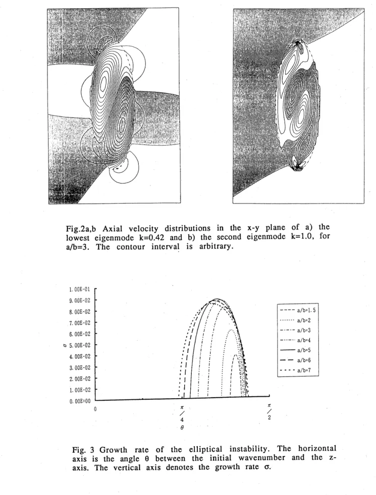
numerical values and the predictions of the elliptical instability.

We show,

as

a

contour map in the x-y plane, the distributions

of the axial velocity of the lowest eigenmode $(k=0.42$

:

Fig $2a)$ and

of the second eigenmode $(k=1.O$

:

Fig $2b)$ for $a/b=3.0$

.

The azimuthal

wavenumber $m$ is 1 inside of the ellipse in both figures. One node

becomes

more

complex

as

the axial wavenumber of the instability

mode increases and that the ith mode has i-l node lines inside of

the ellipse. These figures have resemblance with those of

Pierrehumbert5

(Fig.2) and of

Waleffe7

(Fig.2), indicating the

intimate relation to the elliptical instability

even

at lower modes.

In Fig.$2a$,

we

observe the azimuthal dependence of $m=3$ outside of

the ellipse, which disappears in Fig.$2b$, completely. It may provide

a

possible explanation why the growth rate of the lowest

instability mode is slightly greater than those of higher modes. In

contrast, very small axial velocity, whose azimuthal dependence is characterized by the wavenumber $m=1$_, is found outside of the

vortex in Fig.$2b$

.

The higher modes $(i> 2)$

are

thought to be

confined in the interior of the ellipse, similarly.

4. Relation to the elliptical instability

The numerical results in the previous section demonstrate that

the elliptical instability does play a crucial role in the destabilization of

a

vortex patch of finite extent. The aim of this

section is to give

a

physical interpretation of the theoretical

(asymptotic) results of Vladimirov

&

$I1’in^{21}$ and Tsai

&Widnall2

and the numerical results of Robinson

&

Saffman18, from this stand point.

First,

we

describe the derivation of the values in the last

row

of Tablel, which

are

estimated by the local analysis for the

elliptical instability influenced by a Coriolis force. In the rotating

coordinates, the vorticity inside of the ellipse is reduced to

$\omega’0=(a^{2}+b^{2})/(a+b)^{2}$ and the Rossby number (Miyazak$i^{}$ used the

inverse of the usual definition) is $4ab/(a^{2}+b^{2})$

.

The prescription for

the determination of the Floquet exponents is found in

Craik9

and

Miyazakill.

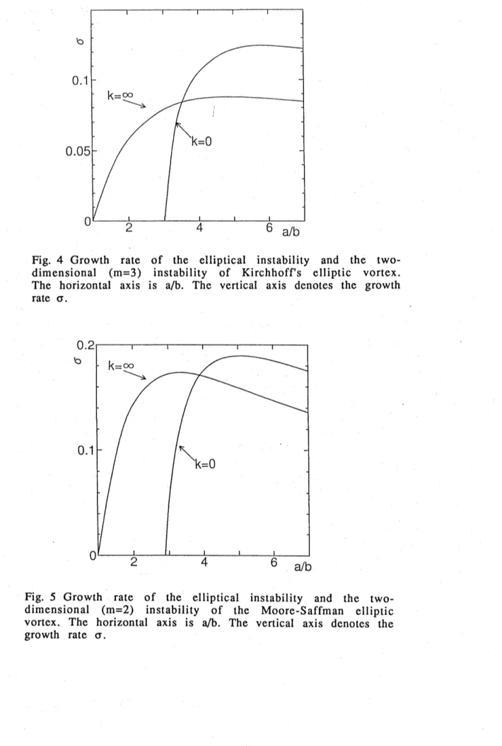
We show the results in Fig.3. The horizontal axis is the

angle 6 between the initial wavenumber vector and the z-axis. The vertical axis is the growth rate $\sigma$ of the instability. Seven

cases

$(a/b=1.5,2.0,3.0,4.0,5.0$ , 6.0 and 7.0$)$

are

figured by

seven

lines

of different type. As $a/b$ is increased, the instability band width

increases and

so

is the maximum growth rate. The latter, however,

saturates and tend to decrease if $a/b$ is increased

over

about 5.0.

The numerical values listed in the bottom of Tablel

are

calculated in this way. It is interesting to note that the value $\Theta=0.3725\pi$ _,

where the maximum is attained for $a/b=3.0$, _has

a

close relation to

the axial velocity profiles in Fig.$2b$

.

If

we

approximate the profile

by $J_{1(\kappa p)}$ ($p=(x^{2}/9+y^{2})^{1/2}$

:

following Waleffe), $\kappa$ is estimated to be

about

6.9

from the fact that the first

zero

of the Bessel function is

$\kappa p=3.83$, which corresponds to _$p=0.55$ in the figure. The value of $\mu$

in

Waleffe7

is equal to $k(=1.O)$

.

Remembering the definition

tan6$=\kappa/3\mu$,

we

have $\Theta=0.37\pi$_, which is close to the above value.

This observation provides another evidence that

our

numerical results

are

closely linked to the elliptical instability.

We plot the maximum growth rate against $a/b$ in Fig.4, where

Love’s two-dimensional $result2$ is included for comparison. It

can

be

seen

that for ellipses with $a/b$ less than about 3.5, the

three-dimensional elliptical instability pre-dominates

over

the

two-dimensional instability.

Next,

we

will revisit the results of Robinson

&Saffman18,

who

investigated the instability of

an

elliptical vortex subject to

a

uniform strain. They found, besides the long-wave mode,

short-wave

instability bands, of which two modes

were

figured in their Fig.3. The maximum growth rate of the two modes is the

same

in

the graphical accuracy and

can

be read

as

$\sigma 1i=0.104$ $(i=1,2)$ for

$a/b=1.5$ and $\sigma 1i=0.153$ $(i=1,2)$ for $a/b=2.0$

.

_{These values}

are

compared with the predictions of the elliptical instability, i.e.,

$\sigma=0.1046$ for $a/b=1.5$ and $\sigma=0.1530$ for _$a/b=2.0$

.

We notice the

remarkable coincidence, again. Only the first short-wave mode is

shown in their Fig.10, whose maximum growth rate is read to be

$\sigma 11=0.180$ for $a/b=4.0$

.

It is greater than the estimate $\sigma=0$

.

1713 of the elliptical instability. The

same

is true of the longest instability mode of Kirchhoffs ellipse. The

reason

for this phenomena is that

the lowest mode is likely to suffer the influence of

two-dimensional instabilities, which become dominant

as

$a/b$ is

increased. We draw, in Fig.5, the growth rate of the elliptical instability $(Pierrehumbert^{5}$ _and $Bayly^{6})$

as a

function of $a/b$

together with the growth rate of the two-dimensional instability ($m=2$

:

Moore

&

Saffman19). The Moore-Saffman ellipse with $a/b$

less than about 3.9 is

more

susceptible to the three-dimensional elliptical instability than to the two-dimensional instability.

Finally,

we

compare

the theoretical results of Tsai $\ Widnal1^{2}$

calculation in the limit of small ellipticity, with the prediction of

the elliptical instability.

Waleffe7

deduced that the growth rate of

the elliptical instability asymptote$s$ to $9/16\epsilon=0.5625\epsilon$ for $\epsilon=a/b-$

$1<<1$

.

This value is close to the results of Tsai $\ Widnal1^{2}$_{, who}

determined the growth rate of the lowest $mod e$ _to be $0.5708\epsilon$ and

that of the second mode to be $0.5695\epsilon$

.

Similarly, the elliptical

instability under the influence of

a

Coriolis force yields the asymptotic growth rate of $[\omega’o(2R_{0}+3)^{2}/32(R_{0}+1)^{2}]\epsilon$, where $\omega’0$ is

the vorticity inside of the ellipse viewed from the rotating coordinate frame and $R_{0}$ denotes the Rossby number.

Remembering that $\Omega=1/4$ in the limit of $a/b->1$ ,

we

have $\omega’0=1-$

$2(1/4)=1/2$ , $R_{0}=(1/4)/(\omega’0/2)$ $=1$ and then the growth rate

$25/256\epsilon=0.0977\epsilon$

.

It again approximates the values $0.993\epsilon$,

$0.1001\epsilon,$ $0.1005\epsilon,$ $0.1009\epsilon$ and $0.1012\epsilon$ obtained by Vladimirov

&

Il’in21

(note that their definition of the parameter $\epsilon$ is different

from

ours

by

a

factor 2). Even in this limiting case, the elliptical

instability does

a

good job.

The two vortex patches of finite extent considered here, i.e.,

Kirchhff’s ellipse and the Moore-Saffman elliptic vortex

are

embedded in

an

irrotational fluid. No

source

of instability is presented outside of the patches, if it

were

not for stagnation

points. Our findings demonstrate that the estimate based

on

the

concept of the elliptical instability gives quite accurate predictions

of the instability growth rate (within

a

few percent), at least, in

these

cases.

More stringent check will be provided if

we

investigate the three-dimensional linear instability of general

Moore-Saffman

vortices19

embedded in

a

uniform background

vorticity field. In this case, possible instability

sources are

presented both inside and outside of the ellipse.

5. Summary and discussions

We have investigated the three-dimensional linear instability

of Kirchhoffs elliptic vortex. Any ellipse, irrespective of the ratio

$a/b$(_$=semi$-major $axis/semi$-minor axis), is shown to be unstable to

the $m=1$ bending $mode$

.

There

are

an

infinite number of instability

bands, whose locations in the limit of small ellipticity coincide

with the asymptotic results by Vladimirov

&

Il$\prime in^{21}$

.

The width of

$a/b$ and the axial wavenumber $k$ increase. The maximum growth

rate of each band (except for that of the lowest mode) is estimated

by the prediction based

on

the elliptical instability accurately. The

structure of eigenmode in the x-y plane becomes

more

complex

as

the axial wavenumber increases (for the i-th mode, i-l node lines

are

presented inside of the ellipse). The profile of the axial velocity (especially,

near

the center of the vortex) _{resembles that}

of the elliptical instability. This mechanism predominates

over

the

two-dimensional instability for smaller values of $a/b$

.

We _{have reconsidered both the asymptotic results of Tsai}

_&

Widnall2

and Vladimirov

&

$\Pi’in^{21}$ and the numerical results of

Robinson

&

Saffman18, _{from the standpoint of the elliptical}

instability. In every case, _{the values of the instability growth rate} obtained in the earlier studies

are

close to the values predicted by

the elliptical instability.

We speculate through these observations that the concept of the elliptical instability is quite useful in estimating the strength

of three-dimensional bending instabilities of steady isolated

columnar vortices,

even

of finite extent. Since the growth rate of the linear instability is almost independent of the axial

wavelength, the breaking process of Kirchhoff’s elliptic vortex and the Moore-Saffman vortex will be highly sensitive to initial conditions $and/or$ _external noises.

Tablel The maximum growth rate

values predicted by the elliptical listed in the last row.

of each instability band. The instability $(n, karrow\infty)$ are

References

$1_{S.C}$. _{Crow, “Stability theory for} a _{pair of trailing vortices,” AIAA J.} 8, 2172

(1970).

$2_{C.Y}$. _Tsai

and S.E. Widnall, “The stability of short waves on a straight

vonex

flament in a weak extemally imposed strain fiel$d”$ J. Fluid Mech. 73, 721

(1976).

3_{D.W. Moore and P.G. Saffman, “The instability of a straight vortex filament}

in a strain feld.” Proc. R. Soc. London Ser. A346, 415 (1975).

$4_{S.E}$. _{Widnall, D.B. Bliss and C.Y. Tsai, “The instability of short} waves on a

vonex

ring,” J. Fluid Mech. 66, 35 (1974).

$5_{R.T}$. _{Pierrehumbert, “Universal short-wave instability of two-dimensional}

eddies in an inviscid fluid,” Phys. Rev. Lett. 57, 2157 (1986).

$6_{B.J}$. _{Bayly, “Three-dimensional instability of elliptical flow,’l Phys. Rev.}

Lett. 57, 2160 (1986). $7_{F}$.

Waleffe, “On the three-dimensional instability of strained vortices.”

Phys. Flulds A2, 76 (1990).

$8_{M.J}$

.

_{Landman and P.G. Saffman, “The three-dimensional instability of}

strained vortices in a viscous fluid,’t Phys. Fluids 30, 2339 (1987).

$9_{A.D.D}$. _{Craik, ttThe stability of unbounded two- and three- dimensional}

flows subject to body forces: some exact solutions.’t J. Fluid Mech. 198, 275

(1989).

10_{T. Miyazaki and Y. Fukumoto, ttThree-dimensional instability of strained}

vortices in a stably stratified fluid,” Phys. Flulds A4, 2515 (1992).

11_{T. Miyazaki, “Elliptical instability in a stably stratified rotating fluid,1t}

Phys. Fluids A5, 2702 (1993).

$12_{E.B}$. _{Gledzer and V.M. Ponomarev, “Instability of bounded flows with}

elliptical streamlines,’\dagger J. Fluid Mech. 240, 1 (1992).

$13_{S.A}$. _{Orszag and A. Patera, “Secondary instability of wall-bounded shear}

flows,” J. Fluid Mech. 128, ₃₄₇ (1983).

14 T. Herbert, $l$

Secondary instability of plane channel flow to subharmonic three-dimensional disturbances,” Phys. FIuids 26, ₈₇₁ (1983).

15_{B.J. Bayly, S.A. Orszag and T. Herbert, “Instability mechanisms in}

shear-flow transitions,1’ Annu. Rev. Fluid Mech. 20, 359 (1988).

16_{Malkus and F. Waleffe, “Transition from order to disorder in elliptical}

flow: a direct path to shear flow turbulence,t1 Advances in Turbulence 3

17_{R.T. Pierrehumbert and S.E. Widnall, “The two- and three-dimensional} instabilities of a spatially periodic shear layer,” J. Fluid Mech. _114. 59

(1982).

18_{A.C. Robinson and P.G. Saffman, ltThree-dimensional stability of an}

elliptical vortex in a straining field.’t J. Fluid Mech. 142, 451 (1984).

19_{D.W. Moore and P.G. Saffman, “Stmcture of a line vortex in an imposed}

strain,” in _Aircraft Wake Turbulence (ed. Olsen, Goldburg & Rogers,

Plenum, 1971), p. 399.

20_{A.E.H. Love, “On the stability of certain vortex motions.” Proc. London}

Math. Soc. 25, 18 (1893).

21_{V.A. Vladimirov and K.I. $I1’in$, “Three-dimensional instability of an}

elliptic Kirchhoff _vortex.t1 Mech. Zhid. $i$ Gaza3, 40 (1988).

Fig.la-c Instability growth rate

$\sigma=lm(\omega(k))$ for the ellipse of a)

$a/b=1.1,$ $b)a/b=2.0$ and c) _alb$=3.0$. The

horizontal axis is the axial

wavenumber $k$ and the vertical axis is

Fig.$2a,b$ Axial velocity distributions in the x-y plane of a) the

lowest eigenmode $k=0.42$ _and b) the second eigenmode $k=1.O$, for $a/b=3$. The _contour interval is arbitrary.

Fig. 3 Growth rate of the elliptical instability. The horizontal axis is the angle $\Theta$ between the initial wavenumber and the

Fig. 4 Growth rate of the elliptical instability and the

two-dimensional $(m=3)$ instability _{of Kirchhoff’s elliptic vortex.}

The horizontal axis is $a/b$. The vertical axis denotes the growth

rate $\sigma$.

Fig. 5 Growth rate of the elliptical instability and the

two-dimensional $(m=2)$ instability of the Moore-Saffman elliptic

vortex. The horizontal axis is $a/b$. The vertical axis denotes _the