Derivation of Hydrodynamic Limits from either the Liouville Equation or Kinetic Models : Study of an Example (Mathematical Analysis in Fluid and Gas Dynamics)

Derivation of Hydrodynamic Limits from either the Liouville Equation or Kinetic Models:

Study of an Example

BY KAZUO AOKI, CLAUDE BARDOS,

FRAN\cCOIS

GOLSE

&YOSHIO

SONE

dedicated to Seiji Ukai on his 60th birthday Abstract

Hydrodynamic limits can be derived, either formally from the $N$ body Liouville equation,

or from the Boltzmann equation. In the latter case, some mathematical proofs of these derivations have been proposed in the last 20 years. However, both derivations may rely

on

different scaling assumptions and could lead to different equations of state. We first discuss this issue on the derivation of the compressible Euler equation from either the N-body Liouville equation or the Boltzmann equation. Then we study two examples where complete mathematical proofs have been given: the periodic Lorentz gas, and a Knudsen gaswith non classical gas-surface interaction (modeling the impingement of gas molecules on a rough surface).

1. Introduction

The general problem of deriving the physical properties of macroscopic bodies from the microscopic dynamics of its elementary constituents (molecules, ions, atoms...) has been the drivingforceleading tothe foundation of statistical mechanics. More precisely, it

seems

that this very basic and general question received a mathematical formulation only after the pioneering achievements of Maxwell and Boltzmann in the kinetic theory ofgases. Yet, the status of the kinetic theory of gases in the derivation of the macroscopic limits from microscopic first principle dynamics is ambiguous. Indeed, the Boltzmann equation can be derived rigorously from the classical dynamics of a large number of hard spheres of vanishingly small radius. Also, the classical modelsof fluidmechanicscan be derived, more or less rigorously ffom the Boltzmann equation. However, to this date, there is no direct derivation of the Euler or Navier-Stokes equations fiiom the classical $N$ body problem,

and the existing attempts at formal derivations of these models sometimes lead to local equilibrium states and equations of states that may be noticeably different ffom the

ones

In the present paper, we propose a few examples of this situation. In section 2, we show how a formal derivation of the compressible Euler equation from the $N$-body Liouville

equation may lead to different equations of state than the perfect gas pressure law which one gets in the derivation from the Boltzmann equation. In sections 3 and 4, we discuss two examples of particle systems the macroscopic behavior of which is described by

a

diffusion equation that can be derived either directly from the particle system

or

from a kinetic model describing its mesoscopic dynamics. However, eventhoughboth the original particlesystem orthe kinetic model lead to the

same

type of macroscopic equation, namely a diffusion equation, the diffusion coefficients obtained from both derivations happen to be different. Thus, kinetic models sometimes may fail to capture the correct macroscopic dynamics of particles systems.

Nevertheless,

even

ifthe mathematical theory of gas dynamics remains the

source

of

some

of the most challenging open problems in mathematics,

we

have gained

some

partial

un-derstanding of this question of macroscopic limits. Undoubtedly, the progress made in the last

25

years in the mathematical theory of the Boltzmann equation paved the way to the theory of hydrodynamic limits as it now stands. Seiji Ukai contributed greatly to this progress, by giving the first proof of global existence and uniqueness of

a

solution to the Cauchy problem for the Boltzmann equation [U]. Therefore, we offer this little essay to our friend and colleague in recognition of the influence that his scientific achievements have had on some ofthe topics touched here.

2. The Euler Limit

Consider a gas made of $N$ like particles of mass $m$ the motion of which is described

by Newton’s law of Mechanics expressed in the form of the Hamilton equations for the Hamiltonian function given by

$H_{N} \equiv\frac{1}{2}m\sum_{i=1}^{N}|v_{i}|^{2}+m^{2}\sum_{1\leq i<j\leq N}\Phi(|x_{i}-x_{j}|)$, (2.1)

where $\Phi$ :

$\mathrm{R}_{+}^{*}arrow \mathrm{R}_{+}^{*}$ is a smooth nonincreasing function (so that the interparticle force is indeed repulsive).

First pick a length scale $\sigma$ for the apparent radius of the particles. One way of doing this is by first prescribingavelocity scale $c$(that one canthink ofasthe mean thermal speed of

the gas) and define $\sigma$ by the formula $2m\Phi(\sigma)=c^{2}$. With this apparent radius so defined, the potential is rescaled

as

follows:

$m \Phi(r)=U(\frac{r}{\sigma})$ , $r>0$, (2.2)

where $U$ : $\mathrm{R}_{+}^{*}arrow \mathrm{R}_{+}^{*}$

.

Next think ofall theseparticles

as

moving in the whole space $\mathrm{R}^{3}$, with

a

referencevolume

$\mathcal{V}$ which sets the macroscopic length scale to $\mathcal{V}^{1/3}$. Intuitively, the mean free path of

these particles should be

a

length scale that is inversely proportional to the number of particles per unit volume times the cross section of each individual particle; this suggests the formula

mean free path $= \frac{\mathcal{V}}{N\pi\sigma^{2}}$ . (2.3) Another natural notion is that of “packed volume” occupied by the gas (i.e. the sum of the volumes occupied by each molecule viewed as a hard sphere ofradius $\sigma$):

packed volume $=N \frac{4}{3}\pi\sigma^{3}$ (2.4)

Thus we can define a dimensionless number $R$ by the formula

$R= \frac{\mathrm{p}\mathrm{a}\mathrm{c}\mathrm{k}\mathrm{e}\mathrm{d}\mathrm{v}\mathrm{o}\mathrm{l}\mathrm{u}\mathrm{m}\mathrm{e}}{\mathcal{V}}=\frac{4}{3}\frac{\sigma}{\mathrm{m}\mathrm{e}\mathrm{a}\mathrm{n}\mathrm{f}\mathrm{r}\mathrm{e}\mathrm{e}\mathrm{p}\mathrm{a}\mathrm{t}\mathrm{h}}$. (2.5) Westudy macroscopiclimitsof the system of particles above by keeping the volume $\mathcal{V}$fixed,

letting $Narrow\infty$ and $\sigmaarrow 0$. However these assumptions are compatible with _{$Rarrow R_{*}$} with

Consider now the Liouville equation for $F_{N}\equiv F_{N}(t, x_{1}, v_{1}, \ldots, x_{N}, v_{N})$ (the $N$ particle

distribution function):

$\partial_{t}F_{N}+\sum_{1\leq i\leq N}v_{i}\cdot\nabla_{x_{i}}F_{N}=\frac{1}{2}\sum_{1\leq i\leq N}(\sum_{1\leq j\neq i\leq N}\frac{1}{\sigma}U’(\frac{|x_{i}-x_{j}|}{\sigma})\frac{x_{i}-x_{j}}{|x_{i}-x_{j}|})\cdot\nabla_{v_{i}}F_{N}(2.6)$

with an initial data

$F_{N}(0, x_{1}, v_{1}, \ldots, x_{N}, v_{N})=F_{N}^{in}(x_{1}, v_{1}, \ldots, x_{N}, v_{N})$ (2.7)

which is symmetrical in all the particle coordinates in phase space. In other words, it is assumed that, for any permutation $\tau$ of $\{1, \ldots, N\}$,

$F_{N}^{in}(x_{1}, v_{1}, \ldots, x_{N}, v_{N})=F_{N}^{in}(x_{\tau(1)}, v_{\tau(1)}, \ldots, x_{\tau(N)}, v_{\tau(N)})$

.

(2.8)

It is easily seen that this symmetry is preserved by the Hamiltonian flow

so

that for all $t>0$ and all $x_{1},$$v_{1},$ $\ldots$ ,$x_{N},$$v_{N}$,

$F_{N}(t, x_{1}, v_{1}, \ldots, x_{N}, v_{N})=F_{N}(t, x_{\tau(1)}, v_{\tau(1)}, \ldots, x_{\tau(N)}, v_{\tau(N)})$

.

(2.9)

Next introduce the marginals of the density $F_{N}$:

$F_{N}^{k}(x_{1}, v_{1}, \ldots, x_{k}, v_{k})=$

$\int F_{N}^{k}(x_{1}, v_{1}, \ldots, x_{k}, v_{k}, x_{k+1}, v_{k+1}, \ldots, x_{N}, v_{N})dx_{k+1}dv_{k+1}\ldots dx_{N}dv_{N}$ ; (2.10)

The formal derivation ofthe Eulec equation outlined below requires only partial informa-tion concerning the marginals of the $N$-particle distribution $F_{N}$

.

In particular, we try to

delineate the minimal set of assumptions needed for this derivation.

First, the equation for the first marginal, can be obtained from (2.6) by integration in all variables but $t,$ $x_{1}$ and $v_{1}$:

$\partial_{t}F_{N}^{1}+v_{1}\cdot\nabla_{x_{1}}F_{N}^{1}=\frac{1}{2}(N-1)\nabla_{v_{1}}\cdot\int\frac{1}{\sigma}U’(\frac{|x_{1}-x_{2}|}{\sigma})\frac{x_{1}-x_{2}}{|x_{1}-x_{2}|}F_{N}^{2}(t, x_{1}, v_{1}, x_{2}, v_{2})dx_{2}dv_{2}$

.

(2.11) In order to obtain local conservation laws for macroscopic quantities,

one

multiplies (2.11) successively by 1, $v_{1}$ and $\frac{1}{2}|v_{1}|^{2}$, and integrate in $v_{1}$, which leads to local conservation laws for the moments of $F_{N}^{1}$ of order less than or equal to 2.

At this point the importance of the scaling appears and, following the beautiful analysis due to Morrey [Mo], one introduces a “fast ” _{variable $\xi=(x_{2}-x_{1})/\sigma$ and define}

a

new

2-point distribution function by the formula

$G_{N}^{2}(t, x_{1}, v_{1}, \xi, v_{2})=F_{N}^{2}(t, x_{1}, v_{1}, x_{1}+\sigma\xi, v_{2})$ . (2.12)

In terms of $G_{N}^{2}$, the local conservation laws ofmass, momentum and energy

are

$\partial_{t}\int F_{N}^{1}dv_{1}+\nabla_{x_{1}}\cdot\int v_{1}F_{N}^{1}dv_{1}=0$

,

(2.13)

$\partial_{t}\int v_{1}F_{N}^{1}dv+\nabla_{x_{1}}\cdot\int v_{1}\otimes v_{1}F_{N}^{1}dv_{1}=$

$- \frac{1}{2}(N-1)\sigma^{3}\iiint\frac{1}{\sigma}U’(|\xi|)\frac{\xi}{|\xi|}G_{N}^{2}(t, x_{1}, v_{1}, \xi, v_{2})d\xi dv_{2}dv_{1}$, (2.14)

$\partial_{t}\int\frac{1}{2}|v_{1}|^{2}F_{N}^{1}dv+\nabla_{x_{1}}\cdot\int v_{1}\frac{1}{2}|v_{1}|^{2}F_{N}^{1}dv_{1}=$

$- \frac{1}{2}(N-1)\sigma^{3}\iiint\frac{1}{\sigma}U’(|\xi|)\frac{\xi}{|\xi|}\cdot v_{1}G_{N}^{2}(t, x_{1}, v_{1}, \xi, v_{2})d\xi dv_{2}dv_{1}$. (2.15)

Consider first the right hand side of (2.14). By the symmetry (2.9),

$G_{N}^{2}(t, x_{1}, v_{1}, \xi, v_{2})=F_{N}^{2}(x_{1}, v_{1}, x_{1}+\sigma\xi, v_{2})=F_{N}^{2}(x_{1}+\sigma\xi, v_{2}, x_{1}, v_{1})$

$=G_{N}^{2}(t, x_{1}+\sigma\xi, v_{2}, -\xi, v_{1})$

(2.16) Thus

$\iiint\frac{1}{\sigma}U’(|\xi|)\frac{\xi}{|\xi|}G_{N}^{2}(t, x_{1}, v_{1}, \xi, v_{2})d\xi dv_{2}dv_{1}$

$= \iiint-\frac{1}{\sigma}U’(|\xi|)\frac{\xi}{|\xi|}G_{N}^{2}(t, x_{1}-\sigma\xi, v_{2}, \xi, v_{1})d\xi dv_{2}dv_{1}$

$= \iiint-\frac{1}{\sigma}U’(|\xi|)\frac{\xi}{|\xi|}G_{N}^{2}(t, x_{1}-\sigma\xi, v_{1}, \xi, v_{2})d\xi dv_{2}dv_{1}$

$= \frac{1}{2}\int\int\int U’(|\xi|)\frac{\xi}{|\xi|}[\frac{G_{N}^{2}(t,x_{1},v_{1},\xi,v_{2})-G_{N}^{2}(t,x_{1}-\sigma\xi,v_{1},\xi,v_{2})}{\sigma}]d\xi dv_{2}dv_{1}$

.

(2.17) Ifthe families $F_{N}^{1}$ and $G_{N}^{2}$ satisfy the following condition

$(1+|v_{1}|^{2})F_{N}^{1}$ is relatively compact in $w- L_{t}^{\infty}(L_{x_{1},v_{1}}^{1})$

then, up to extraction ofa subsequence, $F_{N}^{1}arrow F^{1}$ and $G_{N}^{2}arrow G^{2}$ as $Narrow+\infty$ and

$\frac{1}{2}\int\int\int U’(|\xi|)\frac{\xi}{|\xi|}[\frac{G_{N}^{2}(t,x_{1},v_{1},\xi,v_{2})-G_{N}^{2}(t,x_{1}-\sigma\xi,v_{1},\xi,v_{2})}{\sigma}]d\xi dv_{2}dv_{1}$

$arrow\frac{3}{16\pi}R_{*}\nabla_{x}\cdot\iiint U’(|\xi|)\frac{\xi\otimes\xi}{|\xi|}G^{2}(t, x_{1}, v_{1}, \xi, v_{2})d\xi dv_{2}dv_{1}$

.

Eventually,

$\partial_{t}\int v_{1}F_{N}^{1}dv+\nabla_{x_{1}}\cdot\int v_{1}\otimes v_{1}F_{N}^{1}dv_{1}=$

$\frac{3}{16\pi}R_{*}\nabla_{x}\cdot\iiint U’(|\xi|)\frac{\xi\otimes\xi}{|\xi|}G^{2}(t, x_{1}, v_{1}, \xi, v_{2})d\xi dv_{2}dv_{1}$

.

(2.19)

The right hand side of (2.15) is handled by

a

similar procedure,

as follows.

First integrate the Liouville equation (2.6) in all variables but $t,,$ $x_{1}$ and $x_{2}$:

$\partial_{t}\iint F_{N}^{2}dv_{1}dv_{2}+\nabla_{x_{1}}\cdot\iint v_{1}F_{N}^{2}dv_{1}dv_{2}+\nabla_{x_{2}}\cdot\iint v_{2}F_{N}^{2}dv_{1}dv_{2}=0$

.

(2.20)

Multiply then (2.20) by $U( \frac{|x_{1}-x_{2}|}{\sigma})$ and integrate in $x_{2}$:

$\partial_{t}\int\int\int U(\frac{|x_{1}-x_{2}|}{\sigma})F_{N}^{2}dx_{2}dv_{1}dv_{2}+\nabla_{x_{1}}\cdot\int\int\int v_{1}U(\frac{|x_{1}-x_{2}|}{\sigma})F_{N}^{2}dx_{2}dv_{1}dv_{2}=$

$\frac{1}{\sigma}\iiint U’(\frac{|x_{1}-x_{2}|}{\sigma})(v_{1}-v_{2})\cdot\frac{x_{1}-x_{2}}{|x_{1}-x_{2}|}F_{N}^{2}(t, x_{1}, v_{1}, x_{2}, v_{2})dx_{2}dv_{1}dv_{2}$

which can be recast in terms of$G_{N}^{2}$ as

$\partial_{t}\iiint U(|\xi|)G_{N}^{2}d\xi dv_{1}dv_{2}+\nabla_{x_{1}}\cdot\iiint v_{1}U(|\xi|)G_{N}^{2}d\xi dv_{1}dv_{2}=$

$\frac{1}{\sigma}\iiint U’(|\xi|)(v_{1}-v_{2})\cdot\frac{\xi}{|\xi|}G_{N}^{2}(t, x_{1}, v_{1}, \xi, v_{2})d\xi dv_{1}dv_{2}$ (2.21)

Substituting (2.21) in (2.15) gives

$\partial_{t}[\int\frac{1}{2}|v_{1}|^{2}F_{N}^{1}dv+\frac{1}{4}(N-1)\sigma^{3}\iiint U(|\xi|)G_{N}^{2}d\xi dv_{1}dv_{2}]$

$- \frac{1}{4}(N-1)\sigma^{3}\iiint\frac{1}{\sigma}U’(\frac{|\xi|}{\sigma})\frac{\xi}{|\xi|}\cdot(v_{1}+v_{2})G_{N}^{2}(t, x_{1}, v_{1}, \xi, v_{2})d\xi dv_{2}dv_{1}$ . (2.22)

Ifthe condition (2.18) is strengthened into

$(1+|v_{1}|^{3})F_{N}^{1}$ is relatively compact in $L_{t}^{\infty}(L_{x_{1},v_{1}}^{1})$

$(|\xi||U’(|\xi|)|+U(|\xi|))(1+|v_{1}|+|v_{2}|)]G_{N}^{2}$ is relatively compact in $w- L_{t}^{\infty}(L_{x_{1},v_{1},\xi,v_{2}}^{1})$

(2.23) then, again up to extraction ofa subsequence, $G_{N}^{2}arrow G^{2}$ as $Narrow+\infty$ and, by the

same

symmetry trick as in (2.17)

$\partial_{t}[\int\frac{1}{2}|v_{1}|^{2}F^{1}dv+\frac{3}{16\pi}R_{*}\iiint U(|\xi|)G^{2}d\xi dv_{1}dv_{2}]$

$+ \nabla_{x_{1}}\cdot[\int v_{1}\frac{1}{2}|v_{1}|^{2}F^{1}dv_{1}+\frac{3}{16\pi}R_{*}\iiint v_{1}U(|\xi|)G^{2}d\xi dv_{1}dv_{2}]$

$=- \frac{3}{32\pi}R_{*}\nabla_{x_{1}}\cdot\iiint U’(|\xi|)\frac{\xi\otimes\xi}{|\xi|}\cdot(v_{1}+v_{2})G^{2}(t, x_{1}, v_{1}, \xi, v_{2})d\xi dv_{2}dv_{1}$

.

(2.24)

At this point, the Euler system for compressible fluids can be derived ffom the system

$(2.13)-(2.19)-(2.24)$ _under a closing assumption on $F_{1}$ and $G^{2}$ which we discuss below.

The classical continuity equation

$\partial_{t}\rho+\nabla_{x_{1}}$$(p\mathrm{u})=0$ (2.25)

follows directly from (2.13) without any further assumption, by defining the macroscopic density $\rho$ and bulk velocity $u$ by

$\int F^{1}(t, x_{1}, v_{1})dv_{1}=\rho(t, x_{1})$ , $\int v_{1}F^{1}(t, x_{1}, v_{1})dv_{1}=\rho u(t, x_{1})$

.

(2.26)

The closure proposed here in order to write the momentum and energy equations consists in assuming that

$F^{1}(t, x_{1}, v_{1})= \frac{\rho(t,x_{1})}{(2\pi\theta(t,x_{1}))^{3/2}}\exp(-\frac{|v_{1}-u(t,x_{1})|^{2}}{2\theta(t,x_{1})})$ (2.27)

i.e. that $F^{1}$ is a local Maxwellian, while $G^{2}$ is of the form

$\frac{\rho(t,x_{1})}{(2\pi\theta(t,x_{1}))^{3}}C(|\xi|, \theta(t, x_{1}))\exp(-\frac{|v_{1}-u(t,x_{1})|^{2}+|v_{2}-u(t,x_{1})|^{2}+2U(|\xi|)}{2\theta(t,x_{1})})$ (2.28)

Then one finds that

$\partial_{t}(pu)+\nabla_{x_{1}}(\rho u\otimes u)+\nabla_{x}p=0$ (2.29)

with a pressure law given by

$p= \rho[\theta-\frac{1}{16\pi}R_{*}\iiint U’(|\xi|)|\xi|C(|\xi|, \theta)e^{-\frac{U(|\text{\’{e}}|)}{\theta}}]$ (2.30)

Now the energy equation reads

$\partial_{t}E+\nabla_{x}\cdot[u(E+p)]=0$ (2.31)

with energy density

$E=p[ \frac{1}{2}|u|^{2}+\frac{3}{2}\theta+\frac{3}{16\pi}R_{*}\iiint U(|\xi|)C(|\xi|, \theta)e^{-\frac{U(|\xi|)}{\theta}}d\xi]$ (2.32)

Thus, wehavederivedthe compressible Euler system $(2.25)-(2.29)-(2.31)$ withthe equation of state $(2.30)-(2.32)$_{, under assumption (2.23). Notice that, if} $R_{*}=0$, the equation of

state $(2.30)-(2.32)$ reduces to the usual perfect gas law

$p=\rho\theta$ , $E= \rho[\frac{1}{2}|u|^{2}+\frac{3}{2}\theta]$ (2.33)

It is particularly remarkable that this compressible Euler system for perfect gases can (un-der certain regularity assumptions, see [Ni], [Ca]$)$ be derived fromthe Boltzmann equation, for example in the

case

of a hard sphere gas. The compressible Euler limit of the Boltz-mann equation does not depend on the kind ofparticle interaction considered (cutoff hard potentials

–see

[Ce] p.

67-71

for this terminology –or hard sphere gases formally

con-verge to the

same

Euler limit).

At

this point, it may be worthwhile to recall that the Boltzmann equation has been rigorously derived from the classical dynamics of a gas of$N$

hard spheres of radius $\sigma$ in the so-called Boltzmann-Grad limit, which

means

that

$Narrow+\infty$ and $\sigmaarrow 0$, with $\frac{N\pi\sigma^{2}}{\mathcal{V}}arrow\frac{1}{l}\in \mathrm{R}_{+}^{*}$

.

(2.33) In the terminology of $(2.3)-(2.5)$, this corresponds to the scaling where

The compressible Euler limit of the Boltzmann equation is obtained under the scaling assumption that the Knudsen number, defined

as

the ratio of the

mean

free path to

a

macroscopic length scale of the flow (which can for example be taken as $\mathcal{V}^{1/3}$)

$Kn= \frac{l}{\mathcal{V}^{1/3}}arrow 0$

.

(2.35)

However, there is a double asymptotics in this type of derivation (from particles to Boltz-mann and then to the compressible Euler system) which prevents from considering the

case

where $\sigma\sim l$ as _{$Narrow+\infty$} and $\sigmaarrow 0$.

Next we discuss

our

closure assumption (2.33). The limiting form $G^{2}$ is suggested by

looking at Gibbs distributions for the $N$ particle system. Observe indeed that, since the

Hamiltonian (2.1) is invariant under the translations

$x_{1}\vdasharrow X+x_{1}$

,

...

, $x_{N}\mapsto X+x_{N}$ ,

it commutes with the total momentum density

$m \sum_{i=1}^{N}v_{i}$

.

In particular, a class of special equilibrium solutions of the Liouville equation (2.6) is given by the formula below (which can be referred to

as

an absolute Gibbs ansatz with parameters $\rho>0,$ $\theta>0$ and $u\in \mathrm{R}^{3}$)

$F_{N}(x_{1}, v_{1}, \ldots, x_{N}, v_{N})=\frac{\rho}{(2\pi\theta)^{3N/2}}\exp[\frac{1}{2\theta}(\sum_{i=1}^{N}|v_{i}-u|^{2}+2\sum_{1\leq i<j\leq N}U(\frac{|x_{i}-x_{j}}{\sigma}))]$

(2.36) and a straightforward computation shows that

$G_{N}^{2}(x_{1}, v_{1}, \xi, v_{2})=\frac{\rho}{(2\pi\theta)^{3}}C_{N}(\theta, |\xi|)\exp[\frac{1}{2\theta}(|v_{1}-u|^{2}+|v_{2}-u|^{2}+2U(|\xi|))]$ (2.37)

with

$C_{N}( \theta, |\xi_{2}|)=\int\sigma^{3(N-2)}\exp[\frac{1}{\theta}(\sum_{j=3}^{N}U(|\xi_{j}|)+\sum_{2\leq i<j\leq N}U(|\xi_{i}-\xi_{j}))]d\xi_{3}\ldots d\xi_{N}$ .

In particular,

$F_{N}^{1}(x_{1}, v_{1})= \frac{\rho}{(2\pi\theta)^{3/2}}e^{-\frac{|v_{1}-u|^{2}}{2\theta}}\int\sigma^{3}C_{N}(\theta, |\xi|)e^{-\frac{U(|\xi|)}{\theta}}d\xi$

.

(2.39)

Therefore, in order to be consistant with (2.23), an absolute Gibbs distribution parame-trized by $p>0,$ $\theta>0$ and $u\in \mathrm{R}^{3}$ should satisfy the conditions

$\int\sigma^{3}C_{N}(\theta, |\xi|)e^{-\frac{U(|\xi|)}{\theta}}d\xiarrow 1$ (2.40)

as

well

as

$\int[U(|\xi|)+|\xi||U’(|\xi|)|]C_{N}(\theta, |\xi|)e^{-\frac{U(|\xi|)}{\theta}}d\xiarrow\int[U(|\xi|)+|\xi||U’(|\xi|)|]C(\theta, |\xi|)e^{-\frac{U(|\xi|)}{\theta}}d\xi$

(2.41) as $Narrow+\infty$ (and $\sigmaarrow 0$ with $N\sigma^{3}arrow R_{*}$). One can check that there is

no

contradiction

between (2.40) and (2.41). For example, if

$C_{N}(\theta, |\xi|)e^{-\frac{U(|\xi|)}{\theta}}=\chi(\sigma|\xi|)$

and

$U(|\xi|)=|\xi|^{-3}$

or

if $U\in C_{c}^{0}(\mathrm{R}_{+})$

with

$\chi\geq 0$

,

$\int\chi(|\xi|)d\xi=1$ , and $\int|\xi|^{-3}\chi(|\xi|)d\xi,$ $+\infty$

.

one finds that (2.40) holds, while (2.41) becomes

$\int[U(|\xi|)+|\xi||U’(|\xi|)|]\chi(\sigma|\xi|)d\xiarrow-2\int|\xi|^{-3}\chi(\xi)d\xi$

in the first

case

or

$\int[U(|\xi|)+|\xi||U’(|\xi|)|]\chi(\sigma|\xi|)d\xiarrow\int[U(|\xi|)+|\xi||U’(|\xi|)|]\chi(0)d\xi$

in the second.

The closure assumption proposed in (2.23) consists in restricting

our

attention to

Gibbs

distributions with parameters that areslowly varying in one coordinate, say $x_{1}$

.

We hope

to discuss the possibility of actually constructing such slowly varying Gibbs profiles in a forthcoming publication. Of course, one might think that such a procedure breaks the

symmetry (2.9), which,

as we

have seen in (2.17) and (2.24), is an essential feature of

our

derivation. However, assumption (2.23) bears only

on

the limiting form of $G_{N}^{2}$ as $\sigmaarrow 0$,

in which all particles are collapsed on the same position $x_{1}$.

As a final remark, we just point out the noticeable difference between the form of $G^{2}$

postulated in (2.23) and the fact that, in the Boltzmann-Grad limit, particles

are

supposed to be uncorrelated before collisions. Indeed, the form (2.23) seems to postulate that two neighboringparticles (thatis, particles 1 and 2 with $|x_{1}-x_{2}|$ of order$\sigma$, whichcorresponds to the prescription that $|\xi$ is oforder 1) are correlated independently of whether they are about to collide

or

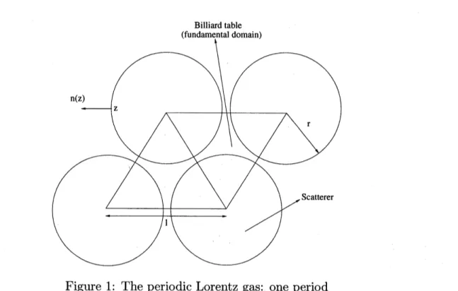
havejust collided.

3. The Periodic Lorentz Gas

In this section and the next one, we leave aside the smooth dynamics of $N$ particles

interacting via a repulsive potential, and consider instead the large scale discontinuous dynamics corresponding to a dispersive billiards system. This goes under the name of Lorentz gas and is an extremely popular class of models in nonequilibrium statistical mechanics:

see

[Sp] for

a

general description.

We

are

concerned here with

a

particular exampleof Lorentz gas. Consider in the euclidian plane $\mathrm{R}^{2}$ the lattice

$\Lambda=\mathrm{Z}(1,0)\oplus \mathrm{Z}(\frac{1}{2}, \frac{\sqrt{3}}{2})$

.

(3.1)

For each positive $\epsilon$ and $r\in$]$0,$ $\frac{1}{2}$[, define $Z(\epsilon, r)$ to be

$Z(\epsilon, r)=$

{

$x\in \mathrm{R}^{2}|$ dist $(x,$$\epsilon k)>\epsilon r$

};

(3.2)

Figure 1: The periodic Lorentz gas: one period

Consider next

a

gas of like point particles moving freely at unit speed in the domain

$Z(\epsilon, r)$.

Assume

further that, upon impinging

on

the boundary of $Z(\epsilon, r)$, these particles

are

specularly reflected and neglect collisions between particles. (That such collisions

can

be neglected at all results from the assumption that the radius of these particles, and therefore their cross section, is zero). This dynamical system is sometimes referred to

as

a “billiard system”, in which case the domain $Z(\epsilon, r)$ is called the “billiard table”. Below,

we denote by $x\in Z(\epsilon, r)$ the positions of the particles, and by $v\in S^{1}$ their velocities.

The billiard system generates, for each positive $\epsilon$, a flow on the one-particle phase space

$Z(\epsilon, r)\cross S^{1}$, denoted by

$(X_{\epsilon}(t;x_{0}, v_{0}),$$V_{\epsilon}(t;x_{0}, v_{0}))$ ; (3.3)

$X_{\epsilon}(t;x_{0}, v_{0})$ is the position at time $t$ofaparticle which, at time $0$ occupied the position $x$

and had instantaneous velocity $v_{0}$, while $V_{\epsilon}(t;x_{0}, v_{0})$ denotes the velocity of this particle.

Clearly, this flow is invariant under translations by lattice vectors, i.e.

$(X_{\epsilon}(t;x_{0}+\epsilon k, v_{0}),$ $V_{\epsilon}(t;x_{0}+\epsilon k, v_{0}))=(X_{\epsilon}(t;x_{0}, v_{0}),$$V_{\epsilon}(t;x_{0}, v_{0}))$ , $k\in\Lambda$, (3.4)

and scales as follows:

$(X_{\epsilon}(t;x_{0}, v_{0}),$ $V_{\epsilon}(t;x_{0}, v_{0}))=(\epsilon X_{1}(t/\epsilon;x_{0}/\epsilon, v_{0}),$$V_{1}(t/\epsilon;x_{0}/\epsilon, v_{0}))$ . (3.5)

In 1981, Bunimovich and Sinai announced the following striking result on this billiard system.

Theorem 3.1. (see $[BSJ$, [BSCJ) Assume that $r$

satisfies

the condition

$\frac{\sqrt{3}}{4}<r<\frac{1}{2}$ , (3.6)

and,

_for

all $(x, v)\in Z(1, r)\mathrm{x}S^{1}$ and all $\epsilon>0$, set

$q_{\epsilon}(t;x, v)=\epsilon X_{1}(t/\epsilon^{2};x, v)$

.

(3.7)

Call $\mu_{\epsilon}$ the probability measure on $C^{0}(\mathrm{R}_{+;}\mathrm{R}^{2})$

defined

as the image

of

the

uniform

prob-ability measure on $(Z(1, r)/\Lambda)\cross S^{1}$ under the map

$(x, v)\mapsto q_{\epsilon}(\cdot;x_{0}, v_{0})$

.

(3.8)

Then$\mu_{\epsilon}$ convergesweakly as $\epsilonarrow 0$ to the Wienermeasure associatedto a Brownian motion

with

_diffusion

matrix

$\sigma^{2}=2E(\tau_{1}(x_{0}, v_{0})^{2}v_{0}\otimes v_{0})+\sum_{k\geq 1}E(\tau_{1}(x_{0}, v_{0})\tau_{1}(x_{k}, v_{k})v_{0}\otimes v_{k})$ (3.9)

where

$\bullet$ the expectation is taken with respectto theprobability

measure

proportionalto $v\cdot n_{1}(x)dvdx$

$on$

$\Gamma_{+}=\{(x_{0}, v_{0})\in(\partial Z(1, r)/\Lambda)\cross S^{1}|v_{0}\cdot n(x_{0})>0\}$ (3.10)

with $n_{1}(x_{0})$ denoting the unit inward normal at point $x_{0}\in\partial Z(1, r)$;

$\bullet$ $\tau_{1}$ is the

forward

exit time, $i.e$.

$\tau_{1}(x, v)=\sup\{t\geq 0|[x, x+tv]\subset Z(1, r)\}$; (3.11)

$\bullet$ the point $(x_{k}, v_{k})$ is the image

of

$(x_{0}, v_{0})$ under the k-th iterate

of

the map

$\Phi$

:

_{$\Gamma_{+}\ni(x, v)rightarrow(x+\tau_{1}(x, v)v,$} $v-2v\cdot n_{1}(x)n-1(x))\in\Gamma_{+}$

.

(3.12)

Bunimovich and Sinai based their discussion on a very intricate construction of Markov partitions with countable alphabet for the map $\Phi$ above. In particular, this construction helps in proving the subexponential decay of velocity correlations

where $C$ and $c$ are two positive constants.

The assumption that $r>\sqrt{3}/4$ implies that the billiard table under consideration has

finitehorizon, which

means

that no particle can

cross

a fundamentaldomain for the action of$\Lambda$

on

$\mathrm{R}^{2}$ without colliding with an obstacle. Thus,

$|\tau_{1}(x, v)|<1$ , for all $(x, v)\in\Gamma_{+}$ . (3.14)

With the above decay (3.13) for the velocity correlations, the bound (3.14) implies that the series defining the diffusion matrix above converges.

These considerations apply to all hyperbolic billiards (see [BSC] for a description of the geometric conditions allowing the application of the theory described above). However, the series (3.9) defining the diffusion coefficient above is neither explicit in the elementary geometric parameters of the billiard table, nor is it very easily computed. Even by taking account of the fast decay of velocity correlations (3.13),

one

should bear in mind that the constants $C$ and $c$

are

not explicit, which makes it hard to predict where the series

can

safely be truncated; also the billiard map $\Phi$ in (3.12), which contains tremendous

instabilities, should be computed for sufficiently many points of $\Gamma_{+}$ to allow the

use

of

quadrature formulas in order to compute the expections involved in the truncated series (3.9).

To avoid this difficulty, it was imagined in [Go] to write a kinetic $\mathrm{e}\mathrm{q}\mathrm{u}\mathrm{a}\mathrm{t}\mathrm{i}\mathrm{o}\dot{\mathrm{n}}$for the above

billiard system by

some

analogy with the Boltzmann-Grad limit, and to subsequently approximate the resulting kinetic equation by

a

diffusion equation,

as

is customary in neutron transport theory, for example. Here is a quick account of this result.

First, write the Liouville equation satisfied by the 1-particle distribution $f_{\epsilon}(t, x, v)$ of

par-ticles in the scaled billiard table:

$\epsilon\partial_{t}f_{\epsilon}+v\cdot\nabla_{x}f_{\epsilon}=0$

,

$x\in Z(\epsilon, r)$ , $v\in S^{1}$ , (3.15)

with the boundary condition expressing that this 1-particle density is invariant under specular reflection at each point of the boundary of $Z(\epsilon, r)$:

$f_{\epsilon}(t, x, v)=f_{\epsilon}(t, x, v-2v\cdot n_{\epsilon}(x)n_{\epsilon}(x))$

,

$x\in\partial Z(\epsilon, r),$ $v\in S^{1}$ (3.16)

Consistently with the notation introduced in Theorem 3.1 above, we denote by $n_{\epsilon}(x_{0})$ the

unit inward normal at the point $x_{0}$ to $\partial Z(\epsilon, r)$

.

This Liouville equation (3.15) and the

associated boundary condition (3.16) are supplemented by

an

initial condition of the form

This Liouville equation (3.15-16) is related to the billiard flow (3.3) defined above by the relation

$f_{\epsilon}(t, x, v)=f_{\epsilon}(t+s, X_{\epsilon}(s/\epsilon;x, v), V_{\epsilon}(s/\epsilon;x, v))$

,

$x\in Z(\epsilon, r),$ $v\in S^{1}$ (3.18)

which,

once

applied to $s=-t$, gives

$f_{\epsilon}(t, x, v)=f^{in}(X_{\epsilon}(t/\epsilon;x, -v))$ , $x\in Z(\epsilon, r),$ $v\in S^{1}$ (3.19)

With the scaling law (3.5) above and the definition (3.7) of$q_{\epsilon}$, this last formula translates

into

$f_{\epsilon}(t, x, v)=f^{in}(q_{\epsilon}(t;x/\epsilon, -v))$, $x\in Z(\epsilon, r),$ $v\in S^{1}$ (3.20)

This last formula should convince the reader discouraged by our shameless introduction ofthe scaling parameter above that studying the limits of solutions of the Liouville

equa-$\mathrm{t}\mathrm{i}\mathrm{o}\dot{\mathrm{n}}$

(3.15-17), and proving that these limits satisfy a diffusion equation, is just a PDE formulation of the Bunimovich-Sinai result in Theorem 3.1 above. Suffice it to say that the small parameter $\epsilon$ can be defined intrinsically as the ratio of the lattice period to the

typical wavelengths present in the Fourier transform of the initial data $f^{in}$.

Asit is, the Liouville equation above (3.15-17) is notany simpler than thebilliard problem, being essentially equivalent to it. An additional difficulty in analyzing the limit of (3.15-3.17) is that the domain

on

where this PDE is posed, namely the billiard table, varieswith

$\epsilon$

.

One

can

remedy to that by extending the 1-particle density $f_{\epsilon}$ by $0$ inside the

$\mathrm{o}\mathrm{b}\mathrm{s}\mathrm{t}\mathrm{a}\mathrm{c}\grave{\mathrm{l}}\mathrm{e}\mathrm{s}$

, i.e. by posing

$F_{\epsilon}(t, x, v)=f_{\epsilon}(t, x, v)$ if $x\in Z(\epsilon, r)$ , (3.21a)

and

$F_{\epsilon}(t, x, v)=0$ if $x\in\overline{Z}(\epsilon, r)^{c}$ (3.21b)

This defines a bona fide distribution (for example, if $f^{in}$ is a bounded function, $F_{\epsilon}$ is

$\mathrm{a}.\mathrm{e}$.

defined and has the same bound

as

$f^{in}$) which satisfies

$\epsilon\partial_{t}F_{\epsilon}+v\cdot\nabla_{x}F_{\epsilon}-(v\cdot n_{\epsilon}(x))\delta_{\partial Z(\epsilon,r)}F_{\epsilon|\partial Z(\epsilon,r)^{i}}=0$ , $x\in \mathrm{R}^{2},$ $v\in S^{1}$ , (3.22)

$F_{\epsilon|\partial Z(\epsilon,r)^{i}}=F_{\epsilon|\partial Z(\epsilon,r)^{i}}\mathrm{o}\mathcal{R}$ $x\in\partial Z(\epsilon, r),$ $v\in S^{1}$ (3.23)

In (3.23), the notation $F_{\epsilon|\partial Z(\epsilon,r)^{i}}$ stands for the trace $F_{\epsilon}$ on $\partial Z(\epsilon, r)$ on the side of$Z(\epsilon, r)$,

while $\mathcal{R}$ designates the transformation

$\mathcal{R}:(t, x, v)-\rangle(t, x, v-2n_{\epsilon}(x)n_{\epsilon}(x))$

.

(3.25)

This relation (3.23)

can

now be used to put (3.22) in the form $\epsilon\partial_{t}F_{\epsilon}+v\cdot\nabla_{x}F_{\epsilon}$

$+(v\cdot n_{\epsilon}(x))_{-}\delta_{\partial Z(\epsilon,r)}F_{\epsilon|\partial Z(\epsilon,r)^{i}}-(v\cdot n_{\epsilon}(x))_{+}\delta_{\partial Z(\epsilon,r)}F_{\epsilon|\partial Z(\epsilon,r)^{i\mathrm{O}}}\mathcal{R}=0$, $x\in \mathrm{R}^{2},$ $v\in S^{1}$

(3.26) This last form should be suggestive to anyone familiar with kinetic equations: indeed the term

$(v\cdot n_{\epsilon}(x))_{-}\delta_{\partial Z(\epsilon,r)}F_{\epsilon|\partial Z(\epsilon_{)}r)^{i}}$ (3.27)

is analogous to the loss term in the Boltzmann collision integral, while the term

$(v\cdot n_{\epsilon}(x))_{+}\delta_{\partial Z(\epsilon,r)}F_{\epsilon|\partial Z(\epsilon,r)^{i}}\circ \mathcal{R}$ (3.28)

is analogousto the gain term in thesameintegral. The onlydifferenceofcourseisthat these terms

are

purely local instead of being integral operators

as

in the

case

ofthe Boltzmann collision operator.

This is remedied in the second step of our approach, explained inthe following Theorem. Theorem 3.2. ([Go]) Consider, the family

_of

operators indexed by $\epsilon>0$

$L$

:

$C^{0}(\mathrm{R}^{2}\cross S^{1})arrow \mathcal{M}(\mathrm{R}^{2}\cross S^{1})$

defined

by

$L_{\epsilon}\phi=(v\cdot n_{\epsilon}(x))_{-}\delta_{\partial Z(\epsilon,r)}\phi_{|\partial Z(\epsilon,r)^{i}}-(v\cdot n_{\epsilon}(x))_{+}\delta_{\partial Z(\epsilon,r)}\phi_{|\partial Z(\epsilon,r)^{i}}\circ \mathcal{R}$ (3.29)

and the operator $L$

defined

by

$(L \phi)(x, v)=\sqrt{3}r(\phi(x, v)-\frac{1}{2}\int_{S^{1}}\phi(x, v’)|v’-v|dv’)$ (3.30)

Then,

_for

any $\phi$ and $\psi\in C_{c}^{\infty}(\mathrm{R}^{2}\cross S^{1})$,

one

has

Thus, instead of considering the transport equation with

measure

coefficients (3.26), one could consider instead

$(1- \frac{2\pi r^{2}}{\sqrt{3}})(\epsilon\partial_{t}G_{\epsilon}+v\cdot\nabla_{x}G_{\epsilon})+\frac{1}{\epsilon}LG_{\epsilon}=0$, (3.32)

which is a much more usualobject. However, Theorem

3.2

says that, for smooth functions $\phi$ independent of$\epsilon,$ $L_{\epsilon}\phi$ and $\frac{1}{\epsilon}L\phi$

are

close to whithin any power of$\epsilon$, but

we

cannot claim

that the same holds true if $\phi$ is replaced by $F_{\epsilon}$.

Nevertheless, this approach shows that one can find a diffusion equation that is close to

the original transport equation with measure coefficients (3.26), in the following sense. Consider $G$ the solution to the diffusion problem

$\partial_{t}G=\frac{1}{2}D(r)\Delta_{x}G$, $x\in \mathrm{R}^{2},$ $t>0$ , (3.33)

$G(\mathrm{O}, x)=f^{in}(x)$

,

$x\in \mathrm{R}^{2}$ , (3.34)

where

$D(r)= \frac{3-2\sqrt{3}\pi r^{2}}{8r}$ _, (3.35)

As is well known, the solution $G$ is smooth for all positive times, and, if$f^{in}$ is assumed to

be smooth, $G$ is smooth all the way down to $t=0$. By the usual theory ofthe diffusion

approximation of transport equation (see for example [BSS]), one

can

construct smooth functions $G_{1}$ and $G_{2}$ of$t,$ $x$ and $v$ such that

$(1- \frac{2\pi r^{2}}{\sqrt{3}})(\partial_{t}+\frac{1}{\epsilon}v\cdot\nabla_{x})(G+\epsilon G_{1}+\epsilon^{2}G_{2})+\frac{1}{\epsilon^{2}}L(G+\epsilon G_{1}+\epsilon^{2}G_{2})=O(\epsilon)_{L^{\infty}}$ (3.36)

while

$(G+\epsilon G_{1}+\epsilon^{2}G_{2})_{|t=0}-f^{in}=O(\epsilon)_{L^{\infty}}$ . (3.37)

Next compute

$( \partial_{t}+\frac{1}{\epsilon}v\cdot\nabla_{x}+\frac{1}{\epsilon}L_{\epsilon})[1_{Z(\epsilon,r)}(G+\epsilon G_{1}+\epsilon^{2}G_{2})]$

$=( \partial_{t}+\frac{1}{\epsilon}v\cdot\nabla_{x})[1_{Z(\epsilon,r)}(G+\epsilon G_{1}+\epsilon^{2}G_{2})]+\frac{1}{\epsilon}L_{\epsilon}(G+\epsilon G_{1}+\epsilon^{2}G_{2})$

$+( \partial_{t}+\frac{1}{\epsilon}v\cdot\nabla_{x})[(1_{Z(\epsilon,r)}-(1-\frac{2\pi r^{2}}{\sqrt{3}}))(G+\epsilon G_{1}+\epsilon^{2}G_{2})]$

$+( \frac{1}{\epsilon}L-\frac{1}{\epsilon^{2}}L_{\epsilon})(G+\epsilon G_{1}+\epsilon^{2}G_{2})=0$

.

(3.38)

Since all the functions $G,$ $G_{1}$ and $G_{2}$

are

smooth,

$( \frac{1}{\epsilon}L-\frac{1}{\epsilon^{2}}L_{\epsilon})(G+\epsilon G_{1}+\epsilon^{2}G_{2})=O(\epsilon^{\infty})_{D’}$ (3.39)

according to Theorem 3.2, while, by the nonstationary phase lemma

one

has

$(1_{Z(\epsilon,r)}-(1- \frac{2\pi r^{2}}{\sqrt{3}}))(G+\epsilon G_{1}+\epsilon^{2}G_{2})=O(\epsilon^{\infty})_{D’}$

.

(3.40)

Thus

we

have proved

Theorem 3.3. $([GoJ)$ Let $G$ be the solution

of

the

diffusion

equation (3.33-34) with

dif-fusion

coefficient

(3.35). Let $G_{1}$ and$G_{2}$ be

defined

as

$G_{1}=-L^{-1}v\partial_{x}G$, $G_{2}=L^{-1}(vL^{-1}v- \frac{1}{2}D(r))\partial_{xx}G$

,

where $L^{-1}$ denotes the pseudo-inverse

of

the Fredholm operator L. Then

$( \partial_{t}+\frac{1}{\epsilon}v\cdot\nabla_{x}+\frac{1}{\epsilon}L_{\epsilon})[1_{Z(\epsilon,r)}(G+\epsilon G_{1}+\epsilon^{2}G_{2})]--O(\epsilon_{D}^{\infty}, +O(\epsilon)_{L^{\infty}}$ (3.41)

Theorem 3.3 shows that replacing the true solution $F_{\epsilon}$ by the truncated asymptotic ex-pansion

$1_{Z(\epsilon,r)}(G+\epsilon G_{1}+\epsilon^{2}G_{2})$ (3.42)

leads to an approximation of the equation (3.26) in the topology of distributions: this corresponds to the notion of consistency.

Comparingthe results in Theorem3.1 and in Theorem 3.3, it

seems

natural to askwhether the diffusion coefficient given by (3.9) coincides with the one computed by the consistent asymptotic expansion (3.42). In other words, does

one

have

In the affirmative, the method based on the search of a consistent asymptotic expansion would lead to avery explicit way of computingthe complicated series (3.9).

However, we cannot infer ffom (3.41) that

$F_{\epsilon}-1_{Z(\epsilon,r)}(G+\epsilon G_{1}+\epsilon^{2}G_{2})arrow 0$

in any reasonable function space. In the language of numerical analysis (referring to the Lax equivalence theorem), this is due to

a

lack ofstability for the transport equation with

measure

coefficients (3.26).

It is interesting to compare this situation with that considered in section 2. As we said, the Boltzmann equation has been rigorously derived from the Liouville equation for a gas of $N$ colliding hard spheres of radius $\sigma$ in the Boltzmann-Grad limit: $Narrow+\infty,$ $\sigmaarrow 0$,

$N\sigma^{2}arrow 1$. The ideas leading to such a derivation are due of Lanford; see [CIP] for a

detailed account ofthe existing proofs. In the case of the Lorentz gas, the kinetic model (3.32) is not proved to be amesoscopiclimit ofthe Liouville equation $(3.15)-(3.16)$ –only the consistency to within any order of accuracy in the

sense

of distributions is established. There

are even

indications that nothing

more

thanconsistency is true:

see

[BGW], [GW].

4. A Model Knudsen Gas

Thus, the example of the periodic Lorentz gas treated in the previous section leads us to

suspect that diffusion coefficients computed by using first a kinetic approximation of the Liouville equation might differ ffomthose computed directly from the definition asthe long time limit of the mean square displacement per unit of time. We say “suspect” because,

as far

as

the periodic Lorentz gas is concerned, we know for sure that both diffusion coefficients differ only in the boring

case

where no diffusion

occurs

really.

In the present section, we analyzeamuch simplerexample, where it is possible to compute explicitly the difference between the diffusion coefficients computed by each method. This example is an amplification ofour previous paper [BGC] (see also [Go2]), which webriefly recall below.

Consider a gas ofpoint particles confined between two infinite plates; as in the

case

of the Lorentz gas, collisions between particles are neglected, for the

same reason

(i.e. because these particles have radius –and therefore cross-section–equal to zero). However, as in the

case

ofthe Lorentz gas,

one

takes into account collisions with the plates. These plates

are

supposed to be rough surfaces, and we shamelessly model the reflection ofparticles

on

the plates by a “chaotic” map, as follows.

Each particle has vertical velocity $\pm 1$ and horizontal velocity $a(\omega)$, where $\omega\in \mathrm{T}^{2}$

.

This variable $\omega$ might look a little obscure, but one could think of $\omega$ as a wave vector in a Brillouin zone and of $a(\omega)$ as the gradient of the energy with respect to this

wave

vector (such models are customary in semiconductors:

see

for example [Po] for a very nice introduction to these models). Anyway, each time a particle travels freely between the plates, which

means

that it keeps not only the

same

horizontal velocity $a(\omega)$, but also the

same

$\omega$

.

Each time

a

particle hits one of the plates, its vertical velocity is changed into its opposite, and its $\omega$ changed into $T\omega$, where $T$ is

a

hyperbolic automorphism of$\mathrm{T}^{2}$, for example

$T=$

$\mathrm{m}\mathrm{o}\mathrm{d}$

.

$2\pi$

.

(4.1)

In what follows, we reduce somewhat the model by assuming that the plates

are

in fact lines. In other words, we suppose that all the values taken by $a$

are

colinear and that

the initial data depends only on the coordinate in the direction of $a$: this symmetry is

preserved by the evolution of the dynamical system considered. The phase space for this system is therefore the cartesian product of the strip $\mathrm{R}\mathrm{x}[0, h]$ by the set parametrizing

velocities i.e. $\mathrm{T}^{2}\cross\{\pm 1\}$, where $h>0$ denotes the distance between the plates. (The set

$\{\pm 1\}$ is just the set of vertical velocities).

Now, as theparticles in this model

move

without seeing each others,

we

might have consid-ered instead a phase space consisting of two copies of the

stri..p

$\mathrm{R}\cross[0, h]$ times $\mathrm{T}^{2}$, where particles going up move on one of the copy while particles going down move

on

the other copy. Ifwe sowthese two strips together along their boundaries, we obtain a cylinder with two marked generatrices

or

seams (see figure 2). Particles

move

on that cylinder

as

follows:

$\bullet$ their angular velocity around the axis of the cylinder is constant (say 1);

$\bullet$ each time

a

particle

crosses one

ofthe two seams, its$\omega$ is changed into$T\omega$ with$T$defined as in (4.1).

In this model, there is an impingement on the “plates” every $h$ unit of time. In order to

observe ahydrodynamic limit, wemust first let $harrow \mathrm{O}$. Since we are interested in observing

adiffusion in the direction of the seams (or the axis of the cylinder), it is natural to assume that $a$ has mean zero

on

$\mathrm{T}^{2}$, and to look at times ofthe order of _$1/h$

.

However, by doing so, we end up with a phase space that shrinks as $harrow \mathrm{O}$ to become $\mathrm{R}\cross \mathrm{T}^{2}$, and we loose

the angle variable.

$\mathrm{H}\cap \mathrm{r}\mathrm{i}7\cap \mathfrak{n}\mathrm{f}\mathrm{f}\mathrm{l}1\tau r\mathrm{e}.\mathrm{l}\mathrm{n}r.\mathrm{i}\mathrm{t}\mathrm{i}\rho..\mathrm{q}$

transrormea

nere

Figure 2: The Knudsen gas model: cylindrical domain.

It is

more

convenient to look instead at the dynamics

on a

$N$-sheet covering of this phase

space with $Narrow\infty$ as $harrow \mathrm{O}$

.

This is done

as

follows:

$\bullet$ the phase space is

$\mathrm{R}\cross S^{1}\cross \mathrm{T}^{2}$;

$\bullet$ each particle has coordinates $(x, \theta, \omega)$ and

moves as

follows: call $\epsilon=\frac{2\pi}{N}$, then

$x’(t)=a(\omega)$

,

$\theta’(t)=1$ , $\omega’(t)=0$, unless $\theta(t)=k\epsilon \mathrm{m}\mathrm{o}\mathrm{d}$

.

$2\pi,$ $k\in \mathrm{Z}$; (4.2a)

in which case, if$\theta(t_{0})=k\epsilon \mathrm{m}\mathrm{o}\mathrm{d}$

.

$2\pi$ with $k\in \mathrm{Z}$, then

The Liouville equation corresponding to this dynamical system is

$\epsilon\partial_{t}f_{\epsilon}-a(\omega)\partial_{x}f_{\epsilon}-\partial_{\theta}f_{\epsilon}=0$, $x\in \mathrm{R},$ $\theta\in S^{1}\backslash \frac{2\pi}{N}\mathrm{Z},$ $t>0$, (4.3)

with the jump condition

$f_{\epsilon}(t, x, k \frac{2\pi}{N}+0, \omega)=f_{\epsilon}(t, x, k\frac{2\pi}{N}-0, T\omega)$ (4.4)

and we

assume

that the initial data is a smooth function of$x$ only, i.e.

$f_{\epsilon}(\mathrm{O}, x, \theta, \omega)=\phi(x)$, $x\in \mathrm{R},$ $\theta\in S^{1}\backslash \frac{2\pi}{N}\mathrm{Z},$ $t>0$

.

(4.5)

In the sequel,

we

denote by brackets

as

in $\langle\cdot\rangle$ the average in $\omega$. The mainresult in [BGC] is as follows

Theorem 4.1. Let $a\in C^{3}(\mathrm{T}^{2})$ be such that $\langle a\rangle=0$

.

Assume that$\phi\in C_{c}^{\infty}(\mathrm{R})$

.

Then

$\bullet$ the

self-correlation

$\langle a\circ T^{n}a\ranglearrow 0$ exponentially

fast

as $narrow+\infty_{i}$ $\bullet$ the absolutely converging series

$D(a)= \sum_{n\in \mathrm{Z}}\langle a\circ T^{n}a\rangle\geq 0$ (4.6)

with equality

_if

and only

_if

$a$ is

a

$L^{2}$ coboundary, $i.e$

. of

the

form

$a=b-b\circ T$ (4.7)

for

some

$b\in L^{2}(\mathrm{T}^{2})$;

$\bullet$ as $\epsilonarrow 0$, the number density $f_{\epsilon}$ converges in $C^{0}([0, \tau], w^{*}-L^{\infty}(\mathrm{R}\cross S^{1}\cross \mathrm{T}^{2}))$

for

all

$\tau>0$ to the solution $f$

of

the

diffusion

equation

$\partial_{t}f=\frac{1}{2}D(a)\partial_{xx}f$, $x\in \mathrm{R},$ $t>0$

,

(4.8)

$f(0, x)=\phi(x)$

,

$x\in \mathrm{R}$

.

(4.9)

Of course, in this case, the diffusion coefficient is not nearly

as

hard to compute

as

in the case ofthe Lorentz gas, in particular because the map $T$ is itself

an

extremely simple

object. For example, if$a$ is a trigonometric polynomial, the series above for $D(a)$ reduces

to a few terms and thus

can

be computed exactly.

Nevertheless, it is instructive to try the detour of a kinetic approximation,

as

outlined in section 3. Going back to the Liouville equation (4.3-5), we patch together all the restrictions of $f_{\epsilon}$ to each connected component of $\mathrm{R}_{t}\cross \mathrm{R}_{x}\cross(S^{1}\backslash \frac{2\pi}{N}\mathrm{Z})_{\theta}\cross \mathrm{T}^{2}$ and call

$F_{\epsilon}$ the function so obtained. This function satisfies the following transport equation

on

$\mathrm{R}_{t}\mathrm{x}\mathrm{R}_{x}\mathrm{x}S_{\theta}^{1}\mathrm{x}\mathrm{T}^{2}$

$\epsilon\partial_{t}F_{\epsilon}+a(\omega)\partial_{x}F_{\epsilon}+\partial_{z}F_{\epsilon}-\sum_{k=1}^{N}\delta(\theta-k\epsilon)[F_{\epsilon|\theta=k\epsilon+0}-F_{\epsilon|\theta=k\epsilon-0}]=0$

.

(4.10)

Averaging this equation in $\theta$ and defining

$G_{\epsilon}(t, x, \omega)=\frac{1}{2\pi}\int_{S^{1}}F_{\epsilon}(t, x, z, \omega)dz$ (4.11)

leads to

$\epsilon\partial_{t}G_{\epsilon}+a(\omega)\partial_{x}G_{\epsilon}-\sum_{k=1}^{N}[F_{\epsilon|\theta=k\epsilon+0}-F_{\epsilon|\theta=k\epsilon-0}]=0$. (4.12)

Next, we use the boundary condition (4.4) to replace the sum above by

$\sum_{k=1}^{N}[F_{\epsilon}(t, x, k\epsilon+0, \omega)-F_{\epsilon}(t, x, k\epsilon-\mathrm{O}, \omega)]=\sum_{k=1}^{N}[F_{\epsilon}(t, x, k\epsilon-\mathrm{O}, T\omega)-F_{\epsilon}(t, x, k\epsilon-\mathrm{O}, \omega)]$

.

(4.13) Now, if$F$ is a smooth function of $\theta$ (which $F_{\epsilon}$ is of

course

not!)

$\sum_{k=1}^{N}[F(t, x, k\epsilon, T\omega)-F(t, x, k\epsilon, \omega)]$

$= \frac{1}{\epsilon}[\int_{S^{1}}F(t, x, z, T\omega)dz-\int_{S^{1}}F(t, x, z, \omega)dz]+O(\epsilon^{\infty})_{D_{\theta}’}$ (4.14)

(see [Go] for what exactly is meant by $O(\epsilon^{\infty})_{D_{\theta}’}$).

In any case,

once

averaged in $\theta$, the Liouville equation (4.3-5) is weakly consistent to

whithin any order of accuracy to the kinetic equation

$g_{\epsilon}(0, x, \omega)=\phi(x)$, $x\in \mathrm{R},$ $\omega\in \mathrm{T}^{2}$ , (4.16)

where $g_{\epsilon}\circ T$ is a shorthand notation for

$(t, x, \omega)\mapsto g_{\epsilon}(t, x, T\omega)$. (4.17)

The proofof consistency to within any order ofaccuracy inthe senseofdistributions rests

on

the Euler-Mc Laurin formula and is as in [Go].

Now we can discuss the limit of (4.15-16) as $\epsilonarrow 0$

.

One finds that the bulk density $\langle g_{\epsilon}\rangle$ is,

in the limit as $\epsilonarrow 0$ governed by a diffusion equation. The proof is not nearly as simple as

the classical proof ofdiffusion approximation inthe case ofthe neutron transport equation because the jump in $\omega$ is purely deterministic. However, thesame kind of techniques

as

in

[BGC] gives the following

Theorem 4.2. Let $a\in C^{3}(\mathrm{T}^{2})$ be such that $\langle a\rangle=0$.

Assume

that $\phi\in C_{c}^{\infty}(\mathrm{R})$

.

Then

as $\epsilonarrow 0$, the family

$g_{\epsilon}$ converges in $L^{\infty}(\mathrm{R}_{+}\cross \mathrm{R}\cross \mathrm{T}^{2}))weak-*to$ the solution

$g$

of

the

diffusion

equation

$\partial_{t}g=\frac{1}{2}D’(a)\partial_{xx}g$, $x\in \mathrm{R},$ $t>0$, (4.18)

$g(0, x)=\phi(x)$

,

$x\in \mathrm{R}$

.

(4.19)

where the

_{diffusion coefficient}

is given by

$D’(a)=2 \sum_{n\geq 0}\langle a\circ T^{n}a\rangle$

.

(4.20)

Sketch

_of

the proof. First one has the following a priori estimates: by the maximum principle

$||g_{\epsilon}||_{L^{\infty}(\mathrm{R}\mathrm{x}\mathrm{R}\cross \mathrm{T}^{2})}+\leq||\phi||_{L\infty(\mathrm{R});}$ (4.21) then, multiplying (4.15) by $g_{\epsilon}$ and integrating in $x$ and $\omega$ (taking account ofthe fact that, by the finite speed of propagation for the transport (4.15) –which is precisely $||a||_{L^{\infty}}/\epsilon$

–each function $g_{\epsilon}$ vanishes at infinity in $x$ as $\phi$ does) one finds

$\frac{1}{2}||g_{\epsilon}(t)||_{L^{2}(\mathrm{R}\cross \mathrm{T}^{2})}+\frac{1}{2\epsilon^{2}}\int_{0}^{t}\int_{\mathrm{R}}\langle g_{\epsilon}-g_{\epsilon}\circ T\rangle dxds=\frac{1}{2}||\phi||_{L^{2}(\mathrm{R})}$

.

(4.22)

Then, one can average the transport equation

4.15

with respect to $\omega$, to find

Next, consider the approximate homological equation for the unknown $b_{\epsilon}\equiv b_{\epsilon}(\omega)$

$\epsilon^{2}b_{\epsilon}+b_{\epsilon}-b\epsilon\circ T^{-1}=a$

.

(4.24)

Since $T$ preserves the Lebesgue

measure

on $\mathrm{T}^{2}$, the operator $a\mapsto a\circ T$ is a unitary transformation of $L^{2}$ and the $b_{\epsilon}$ can be defined by the normally converging series

$b_{\epsilon}= \sum_{n\geq 0}\frac{1}{(1+\epsilon^{2})^{n+1}}a\circ T^{-n}$ (4.25)

Then

$\frac{1}{\epsilon}\langle ag_{\epsilon}\rangle=\langle\epsilon b_{\epsilon}g_{\epsilon}\rangle+\langle b_{\epsilon}\frac{1}{\epsilon}(g_{\epsilon}-g_{\epsilon}\mathrm{o}T)\rangle$

$=\langle\epsilon b_{\epsilon}g_{\epsilon}\rangle-\partial_{t}\langle\epsilon b_{\epsilon}g_{\epsilon}\rangle-\partial_{x}\langle b_{\epsilon}ag_{\epsilon}\rangle$. (4.26) The first equality uses again that the operator $\psi\mapsto\psi\circ T$ is unitaryon $L^{2}(\mathrm{T}^{2})$ with adjoint

$\psi\mapsto\psi\circ T^{-1}$; the second equality

uses

the transport equation(4.15) to replace the $O(1/\epsilon)$

term $\frac{1}{\epsilon}(g_{\epsilon}-g_{\epsilon}\mathrm{o}T)$ by a term involving first order derivatives. Now, we claim that $b_{\epsilon}$ satisfies

$\langle b_{\epsilon}\rangle=0$, $\epsilon\langle b_{\epsilon}^{2}\rangle=O(1)$, (4.27) $\langle b_{\epsilon}a\ranglearrow\frac{1}{2}D’(a)$

as

$\epsilonarrow 0$

.

(4.28)

The first relation in (4.27) is

a

trivial consequence of (4.24); (4.28) follows from the

ex-ponential decay of the self-correlation coefficients of $a$ stated in Theorem 4.1 and the

dominated convergence theorem. As for the second relation in (4.27), one writes

$\epsilon^{2}\langle b_{\epsilon}^{2}\rangle+\langle b_{\epsilon}(b_{\epsilon}-b_{\epsilon}\circ T)\rangle=\langle b_{\epsilon}a\rangle$ (4.29) and

use

that the second term in the left hand side of (4.29) is nonnegative since

$\langle b_{\epsilon}(b_{\epsilon}-b_{\epsilon}\circ T)\rangle=\frac{1}{2}\langle(b_{\epsilon}-b_{\epsilon}\circ T)^{2}\rangle$

.

The last and main step in the proof is provided by the following decorrelation properties: $\langle b_{\epsilon}ag_{\epsilon}\rangle-\langle b_{\epsilon}a\rangle\langle g_{\epsilon}\ranglearrow 0$, (4.30) and

These are obtained from two ingredients. One is the representation ofthe solution$g_{\epsilon}$ as

$g_{\epsilon}(t, x, \omega)=\mathrm{E}\phi(x+\epsilon\sum_{n=0}^{N(t/\epsilon^{2})}\tau_{n}a(T^{n}\omega))$ (4.32)

where $\tau_{n},$ $n=0,$ $\ldots$ is a sequence ofindependent, exponentially distributed random jump

times (i.e. Prob $\{\tau_{n}>t\}=e^{-t}$ for all positive $t$). The other one is the mixing property

enjoyed by $T$ and analogous to the so-called “weak Bernoulli mixing” statedas Proposition

6 of [BGC] (see especially formula (37), p. 43 of [BGC]).

With (4.30) and (4.31), properties (4.27) and (4.28) of$b_{\epsilon}$, plus the weak compactness of the

family $\langle g_{\epsilon}\rangle$ guaranteed by the maximum principle (4.21) show that the family of averages $\langle g_{\epsilon}\rangle$ converges to the solution

$g$ of (4.18-19). Finally, by convexity and weak limit, (4.22)

shows that any $\mathrm{w}\mathrm{e}\mathrm{a}\mathrm{k}-*\mathrm{l}\mathrm{i}\mathrm{m}\mathrm{i}\mathrm{t}$ point of

$g_{\epsilon}$

as

$\epsilonarrow 0$ is invariant under the transformation $T$

acting on the $\omega$ variable. Since $T$ is ergodic, this shows that such $\mathrm{w}\mathrm{e}\mathrm{a}\mathrm{k}-*\mathrm{l}\mathrm{i}\mathrm{m}\mathrm{i}\mathrm{t}$ points

as

$\epsilonarrow 0$ must be independent of$\omega$ and therefore equal to the solution

$g$ of (4.18-19). //

The main interest (if any) ofthis little computation is essentially the following consequence of Theorems 4.1 and 4.2.

Corollary 4.3. For all $a\in C^{3}(\mathrm{T}^{2})$ such that $\langle a\rangle=0$, the $‘ {}^{t}true$”

diffusion coefficient

$D(a)$ and the

diffusion

coefficient

$D’(a)$ computed by the kinetic

theow differ

_by

$D’(a)-D(a)=\langle a^{2}\rangle$

.

(4.33)

In particular, the kinetic theory approach gives a positive diffusion coefficient even if$a$ is

a coboundary. This is completely analogous to the

case

of the Lorentz gas with touching obstacles: in this case, each particle stays confined in the

same

period and the “true” diffusion coefficient is zero. In any case, (4.22) shows that the kinetic model (4.15-16) is dissipative while the Liouville equation is not; thus there should be little surprise in the fact that the diffusion coefficient computed by the kinetic approach is higher than the

References

[BGC] Bardos, C., Golse, F. and Colonna, J. F.: Diffusion approximation and hyperbolic automorphism ofthe torus, Physica D104 (1997),

32-60.

[BSS] Bardos, C., Santos, R., Sentis, R.: Diffusion approximation and computation ofthe critical size; $r_{\mathrm{R}\mathrm{a}\mathrm{n}\mathrm{s}}$

.

Amer. Math. Soc.

284

(1984), no. 2,

617-649.

[BGW] Bourgain, J., Golse, F., Wennberg, B.: On the distributionoffree path lengths for the periodic Lorentz gas; Comm. Math. Phys. 190 (1998), no. 3, 491-508.

[BS] Bunimovich, L. A., Sinal, Ya.

G.:

Statistical Properties of the Lorentz gas with periodic configuration ofscatterers; Comm. Math. Phys.

78

(1981), no. 3,

479-497.

[BSC] Bunimovich, L. A., Sinal, Ya. G., Chernov, N. I.: Statistical properties of two-dimensional hyperbolic billiards; (Russian) Uspekhi Mat. Nauk

46

(1991), no. 4 (280), 43-92, 192; English transl. Math. Surveys

46

(1991), no. 4,

47-106.

[Ca] Caflisch, R.: The fluid dynamic limit of the nonlinear Boltzmann equation; Comm. Pure Appl. Math. 33 (1980), no. 5,

651-666.

[Ce] Cercignani, C.: “The Boltzmann equation and its applications”; Applied Mathemat-ical Sciences, 67. Springer-Verlag, New York, 1988.

[CIP]: Cercignani, C., Illner, R., Pulvirenti, M.: “Themathematicaltheoryof dilute gases”;

Applied Mathematical Sciences, 106; Springer-Verlag, New York,

1994.

[Go] Golse, F.: $r_{\mathrm{b}\mathrm{a}\mathrm{n}\mathrm{s}\mathrm{p}\mathrm{o}\mathrm{r}\mathrm{t}}$ dans les milieux composites fortement contrast\’es I: le mod\‘ele

du billard; Annales Inst. Henri Poincar\’e, Physique Th\’eorique 61 (1994),

381-410.

[Go2] Golse, F.: Diffusion approximation and Arnold’s ”cat map”; Asymptotic modelling in fluid mechanics (Paris, 1994), 179-190, Lecture Notes in Phys., 442, Springer, Berlin,

1995.

[GW] Golse, F., Wennberg, B.: On the distribution of free path lengths for the periodic Lorentz gas II; preprint E.N.S., DMA-99-31.

[Mo] Morrey, C. B.: Onthe Derivation of the Equations of Hydrodynamics from Statistical

Mechanics; Comm. Pure and Appl. Math. 8 (1955), 279-326.

[Ni] Nishida, T.: Fluid dynamical limit of the nonlinear Boltzmann equation to the level ofthe compressible Euler equation; Comm. Math. Phys. 61 (1978), no. 2,

119-148.

[Po] Poupaud, F.: Mathematical theory of kinetic equations for transport modelling in semiconductors; Advances in kinetic theory and computing, 141-168, Ser. Adv. Math.

Appl. Sci., 22, World Sci. Publishing, River Edge, NJ,

1994.

[Sp] Spohn, H. : “Large Scale Dynamics of Interacting Particles”, Texts and Monographs in Physics, Springer-Verlag (1991).

[U] Ukai, S.: On the existence of global solutions of mixed problem for non-linear

Boltz-mann

equation. Proc. Japan Acad.

50

(1974),

179-184.

K.A.

&Y.S.:

KYOTO UNIVERSITY, GRADUATE SCHOOL OF ENGINEERING

DEPARTMENT OF AERONAUTICS AND ASTRONAUTICS, KYOTO 606-8501, JAPAN

C.B.: UNIVERSIT\’E PARIS VII

&E.N.S.

CACHAN, C.M.L.A.

61 AV. DU

PRE’SIDENT

WILSON,

94235

CACHAN CEDEX, FRANCE

F.G.:

_{UNIVE.RSIT\’E}

PARIS VII

&

INSTITUT UNIVERSITAIRE DE FRANCE

ECOLE NORMALE

SUPE’RIEURE,

D.M.A.