Stability analysis of numerical methods for delay integro-differential equations (Discretization Methods and Numerical Algorithms for Differential Equations)

(1)

Stability analysis

of

numerical methods for

delay integr0-differential

equations

TOSHIYUKI Koto 小藤俊幸

Department ofComputer Science

The University of ElectrO-Communications

電気通信大学

e-mail : [email protected]

Abstract

Stability of $\theta$ methods for delay integr0-differential equations (DIDEs) is

studied on the basis ofthe linear equation

$\frac{\mathrm{d}u}{\mathrm{d}t}=\mathrm{X}\mathrm{u}(\mathrm{t})$$+\mathrm{f}\mathrm{i}\mathrm{u}(\mathrm{t} -\tau)$$+ \mathrm{t}\kappa\int_{t-\tau}^{t}u(\sigma)d\sigma$,

where $\lambda$,

$\mu$, $\kappa$ arecomplex numbers and $\tau$ is aconstant delay. It is shown that

every $A$-stable $\theta$-method possesses asimilar stability property to P-stability,

i.e., the method preserves the delay-independent stability of the exact solution under the condition that $\tau/h$ is an integer, where $h$ is astep-size. It is also

shown that the method does not possess the same property if$\tau/h$ is not an

integer. As aresult, any 0-method cannot possess asimilar stability property

to $GP$-stability with respect to DIDEs.

1. Introduction

We study stability of (2-stage)methods fordelay integr0-differential equations

(DIDEs) on the basis of the linear equation

$\frac{\mathrm{d}u}{\mathrm{d}t}=\lambda u(t)+\mu u(t-\tau)+\kappa\int_{t-\tau}^{t}u(\sigma)d\sigma$, (1.1)

where $\lambda$,

$\mu$, $\kappa$ are complex numbers and $\tau$ is aconstant delay. When $\kappa=0$, the

equation (1.1) coincides with the test equation

$\frac{\mathrm{d}u}{\mathrm{d}t}=\lambda u(t)+\mu u(t-\tau)$, (1.2)

which

was

proposed by Barwell [1] to examine stability of numerical methods for

delaydifferential equations (DDEs). As described in [1], if $\lambda$,

$\mu$ satisfy

$|\mu|<-{\rm Re}\lambda$, (1.3)

the zero solution of (1.2) is asymptotically stable for any $\tau\geq 0$

.

This asymptotic

property is called delay-independent stability, and analogous stability properties of

numerical methods are considered on the basis of the condition (1.3). For example

数理解析研究所講究録 1265 巻 2002 年 189-199

(2)

anumerical method for DDEs is said to be $P$-stable if every numerical solution to

(1.2) tends to

zero

whenever $\lambda$,

$\mu$ satisfy (1.3) and $\tau/h$is

an

integer, where $h$ is the

step-size. Anumerical method is said to be $GP$-stable if the

same

holds for any

constant step-size.

In the last two decades, various studies

were

carried out concerning stability

properties of numerical methods for DDEs (see, e.g., [12]). In particular,

an

earliest

study by Watanabe and Roth [10] has revealed that every $A$-stable $\theta$ method is

$GP$-stable. To the contrary, little is known about stability properties of numerical

methods for DIDEs. It isquite recent that we studied delay-independentstability of

linear

DIDEs

[7], and

even

stabilityof$\theta$-methods

for

(1.1) remains to

be

investigated.

By Theorem 2of [7], the zero solution of (1.1) is asymptotically stable for any

$\tau\geq 0$ if and only if $\lambda$,

$\mu$, $\kappa$ satisfy

$\lambda+\mu+\kappa\tau\neq 0$ for any $\tau\geq 0$, (1.1)

$z^{2}-z\lambda-\kappa=0$_, _{$z\in C$}_, _{$z\neq 0$} $\Rightarrow$ ${\rm Re} z<0$, (1.5)

$| \frac{\mu z-\kappa}{z^{2}-z\lambda-\kappa}|<1$ for any ${\rm Re} z=0$ with $z\neq 0$. (1.6)

Moreover, the conditions (1.5), (1.6)

are

rewritten

as

${\rm Re}\lambda<0$ and

(

${\rm Re}$A${\rm Re}(\lambda\overline{\kappa})+({\rm Im}\kappa)^{2}<0$

or

$\kappa=0$

),

(1.7)

${\rm Im}[(\lambda+\mu)\overline{\kappa}]=0$ and $[|\mu|^{2}<({\rm Re}\lambda)^{2}+2{\rm Re}\kappa$

or

(

${\rm Im}\lambda=0$, $|\mu|^{2}=({\rm Re}\lambda)^{2}+2{\rm Re}\kappa$

)

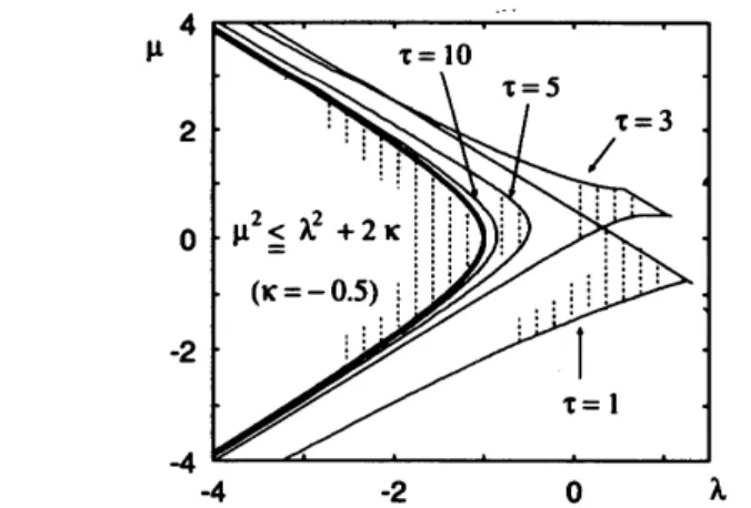
$]$, (1.8)

respectively (Sect. 3in [7]). When $\lambda$,

$\mu$, $\kappa$ are all real and $\kappa\neq 0$, these conditions

are reduced to the simple condition

$\lambda<0$, $\kappa<0$, $\mu^{2}\leq\lambda^{2}+2\kappa$

.

(1.9)

We study stability properties of $\theta$-methods by comparing the region determined by

these conditions with akind of stabilityregions of the methods.

Fig. 1Delay-independent v.s. delay-dependent stability regions

(3)

It

should be noted that

aconsiderable

number of papers [2, 3, 4, 6, 9]

are

devoted

to stability analysis of&-methods for DDEs, which does not

seem

strange from

a

practical viewpoint. Some important instances of stiff DDEs

are

obtained from the

space-descritization of partial functional differential equations (see, e.g., [13]). The

&-methods

have practicality in such asituation.

2. Stability

regions

of $\theta$-methods

Consider delay integr0-differential equations (DIDEs) with aconstant delay,

$\frac{\mathrm{d}u}{\mathrm{d}t}=f$

(

$t$,$u(t)$,$u(t-\tau)$,$\int_{t-\tau}^{t}g(t,$$\sigma$,$u(\sigma))d\sigma$

).

(2.1)

For

agiven step-size $h>0$,

let

$m$ be

the smallest

integer greater than

or

equal to

$\tau/h$. Then, the delay $\tau$ is represented in the form

$\tau=(m-\delta)h$, $0\leq\delta<1$, (2.2)

and the relation

$t_{n}-\tau=t_{n-m}+\delta h$ (2.3)

holds for the step points $t_{n}=t_{0}+nh$, $n\in Z$.

By approximating the delayed argument and the integrand in (2.1) with linear

interpolation, we can adapt a $\theta$-method to (2.1) as follows:

$u_{n+1}=u_{n}+h(1-\theta)f(t_{n}, u_{n}, v_{n}, G_{n})+h\theta f(t_{n+1}, u_{n+1}, v_{n+1}, G_{n+1})$, (2.4)

where, $0\leq\theta\leq 1$, $u_{n}$ is an approximate value of $u(t_{n})$, and

$v_{n}$ $=$ $(1-\delta)u_{n-m}+\delta u_{n-m+1}$, (2.5)

$G_{n}$ $=$ $\frac{h(1-\delta)^{2}}{2}g(t_{n}, t_{n-m}, u_{n-m})+\frac{h(2-\delta^{2})}{2}g(t_{n}, t_{n-m+1}, u_{n-m+1})$

$+h \sum_{k=2}^{m-1}g(t_{n}, t_{n-m+k}, u_{n-m+k})+\frac{h}{2}g(t_{n}, t_{n}, u_{n})$. (2.1)

As aresult, the integral term of (2.1) is approximated with the trapezoidal rule.

When $\theta=1/2$ and $\delta=0$, the formula (2.4)-(2.6) determines amethod that belongs

to aclass of Runge-Kutta methods discussed in [7]. But, when $\theta\neq 1/2$, it gives

another type of numerical method.

In the

case

of the test equation (1.1), the formula (2.4)-(2.6) is reduced to

$u_{n+1}$ $=$ $u_{n}+(1-\theta)\alpha u_{n}+\theta\alpha u_{n+1}$

$+\beta[(1-\delta)(1-\theta)u_{n-m}+(\delta+\theta-2\delta\theta)u_{n-m+1}+\delta\theta u_{n-m+2}]$

$+ \gamma[\frac{(1-\delta)^{2}(1-\theta)}{2}u_{n-m}+\frac{(2-\delta^{2})(1-\theta)+(1-\delta)^{2}\theta}{2}u_{n-m+1}$

$+ \frac{2-\delta^{2}\theta}{2}u_{n-m+2}+\sum_{k=3}^{m-1}u_{n-m+k}+\frac{1+\theta}{2}u_{n}+\frac{\theta}{2}u_{n+1}]$, (2.7)

(4)

$\alpha=h\lambda$

,

_$\beta=h\mu$

,

$\gamma=h^{2}\kappa$

.

The characteristic equation of (2.7) is written as

(2.8)

$z^{m+1}$ $z^{m}-(1-\theta)\alpha z^{m}-\theta\alpha z^{m+1}$

$-\beta[(1-\delta)(1-\theta)+(\delta+\theta-2\delta\theta)z+\delta\theta z^{2}]$

$- \gamma[\frac{(1-\delta)^{2}(1-\theta)}{2}+\frac{(2-\delta^{2})(1-\theta)+(1-\delta)^{2}\theta}{2}z$

$+ \frac{2-\delta^{2}\theta}{2}z^{2}+\sum_{k=3}^{m-1}z^{k}+\frac{1+\theta}{2}z^{m}+\frac{\theta}{2}z^{m+1}]=0$

.

(2.9)

Using (2.9)

we

define the

sets $S_{\theta,m}^{(\delta)}$ and $S_{\theta}^{(\delta)}$

for

_{$0\leq\delta<1$} by

$S_{\theta,m}^{(\delta)}=$

{

$(\alpha$,$\beta$,$\gamma)\in C^{3}$ : all the roots of (2.9) satisfy

$|z|<1$

},

(2.10)

$S_{\theta}^{(\delta)}=\cap S_{\theta,m}^{(\delta)}m\geq 1^{\cdot}$ (2.11)

The set $S_{\theta}^{(\delta)}$ is

an

analogue of the $\delta$-stability region of the $\theta$-method[4].

When $z=1$, the left hand side of (2.9) is equal $\mathrm{t}\mathrm{o}-[\alpha+\beta+(m-\delta)\gamma]$

.

Hence,

for any $m\geq 1$, $z=1$ is not aroot of (2.9) if and only if

$(\mathrm{C}_{0})$ _{$\alpha+\beta+(m-\delta)\gamma\neq 0$} for any _{$m\geq 1$}

.

Substituting $\sum_{k=3}^{m-1}z^{k}=(z^{3}-z^{m})/(1-z)$ into (2.9) and multiplying _$(1-z)$,

we

_get

$z^{m}q(z)-p(z)=0$, _(2.12) $q(z)$ $=$ $q_{0}z^{2}+q_{1}z+q_{2}$, (2.13) $p(z)$ $=p_{0}z^{3}+p_{1}z^{2}+p_{2}z+p_{3}$, _(2.14) where $q_{0}$ $=$ $\theta\alpha+\frac{\theta}{2}\gamma-1$, $q_{1}=(1-2 \theta)\alpha+\frac{\gamma}{2}+2$, $q_{2}$ $=$ $-(1- \theta)\alpha+\frac{1-\theta}{2}\gamma-1$, $p_{0}$ $=$ $- \delta\theta\beta+\frac{\delta^{2}\theta}{2}\gamma$, $p_{1}=(3 \delta\theta-\delta-\theta)\beta+\frac{-3\delta^{2}\theta+\delta^{2}+2\delta\theta+\theta}{2}\gamma$, $p_{2}$ $=$ $(-3 \delta\theta+2\delta+2\theta-1)\beta+\frac{3\delta^{2}\theta-2\delta^{2}-4\delta\theta-2\delta^{2}+2\delta+1}{2}\gamma$, $p_{3}$ $=$ $( \delta\theta-\delta-\theta+1)\beta+\frac{-\delta^{2}\theta+\delta^{2}+2\delta\theta-2\delta-\theta+1}{2}\gamma$

.

Moreover we

set $r(z)=p(z)/q(z)$, (2.15)

and consider the following conditions

(5)

(a) $q(z)\neq 0$ for any

|z

$|\geq 1$

.

(\^a) $q(z)\neq 0$ for any _$|z|>1$.

(b) $|r(z)|<1$ for any $|z|=1$ with $z\neq 1$

.

(b) $|r(z)|\leq 1$ for any _$|z|=1$

.

These are regarded as conditions for $\alpha$, $\beta$,

$\gamma$. We also write

(c) $(\alpha, \beta, \gamma)\in S_{\theta}^{(\delta)}$.

Under this notation, we

can

characterize $S_{\theta}^{(\delta)}$

as

follows.

Theorem 2.1 The following implications hold:

$(\mathrm{C}_{0})$ and (a) and (b) $\Rightarrow$ (c) $\Rightarrow$ (\^a) and (b).

If, in addition,

$(\mathrm{C}_{1})$ $p(z)$, $q(z)$ have

no common zero on

$|z|=1$,

then (c) implies (a).

Proof. Assume $(\mathrm{C}_{0})$, (a) and (b). We first show that $\hat{r}(z)=r(z)/z$ satisfies

$|\hat{r}(z)|<1$ for any $|z|\geq 1$ with $z\neq 1$.

The linear fractional transformation

$z= \frac{w+1}{w-1}$ (2.16)

maps ${\rm Re} w>0$ conformally onto $|z|>1$, with $w=\infty$ corresponding to $z=1$

.

The

function $\hat{R}(w)=\hat{r}[(w+1)/(w-1)]$ is represented in the form

$\hat{R}(w)$ $=$ $\hat{P}(w)/\hat{Q}(w)$, (2.17)

$\hat{P}(w)$ $=$ $[\gamma w^{2}+(-2\beta+2\delta\gamma-\gamma)w+2(1-2\delta)\beta-2\delta(1-\delta)\gamma]$

$\cross[w-(1-2\theta)]$, (2.18)

$\hat{Q}(w)$ $=$ $(w+1)\{\gamma w^{2}+[2\alpha-(1-2\theta)\gamma]w-2(1-2\theta)\alpha-4\}$. (2.19)

Then, itfollowsfrom (a) that $\hat{R}(w)$ is abounded, holomorphic functionin ${\rm Re} w>0$

.

Hence, by the Phragm\’en-Lindel\"of theorem (see, e.g., [8], p. 168), it follows from (b)

that $|\hat{R}(w)|<1$ for any ${\rm Re} w>0$, which implies that $|\hat{r}(z)|<1$ for any $|z|\geq 1$

with $z\neq 1$.

If $|z|\geq 1$ and $z\neq 1$, then

$z^{m}q(z)-p(z)=q(z)z[z^{m-1}-\hat{r}(z)]\neq 0$,

(6)

which, together with $(\mathrm{C}_{0})$, implies (c).

Assume (c). If $q(z_{0})=0$ for

some

$|z_{0}|>1$,

then there

exists $\epsilon>0$ such that

$C(z_{0}, \epsilon)\subset$

{|z

_$|>1\}$

and

$q(z)\neq 0$

on

$C(z_{0},\epsilon)$

, where

$C(z_{0}, \epsilon)=\{z\in \mathcal{O} : |z-z_{0}|=\epsilon\}$

.

By Rouch\’e’$\mathrm{s}$ theorem, the polynomial $z^{m}q(z)-p(z)$ has aroot in the

interior

of

$C(z_{0}, \epsilon)$ for sufficiently large _$m$, which contradicts (c). Therefore, (\^a) holds.

Moreover, if $|r(z_{0})|>1$ for

some

$|z_{0}|=1$, then the equation $z^{m}=r(z)$

has asolution with $|z|>1$ for sufficiently large $m$

.

This is verified by applying

Proposition 7 of [11] to$\psi(z)=1/r(z)$

.

Infact,there exists$\epsilon$ $>0$such that $|r(z)|>1$

for any $z\in\overline{V_{\epsilon}}$, where _{$V_{\epsilon}=\{z\in \mathcal{O} :} _{|z-(1+\epsilon)z_{0}|<\epsilon\}$}

.

Hence, $\rho=\mathrm{m}_{\frac{\mathrm{a}\mathrm{x}}{V_{e}}}|\psi(z)z\in|<1$

,

and $1\in ae\backslash B(0, \rho)$, where _{$B(0, \rho)=\{z\in C : |z|\leq\rho\}$}

.

On the other hand,

we

have

$\mathcal{O}\backslash B(0, \rho)\subset\cup\{z^{m}\psi(z)m\geq 1$: z

$\in V_{\epsilon}\}$, (2.20)

by Proposition 7of [11]. Since $|z|>1$ for any $z\in V_{\epsilon}$, it follows from (2.20) that

$z^{m}=r(z)$ holds for

some

$m\geq 1$ and _$|z|>1$, which contradicts (c). Therefore, $(\hat{\mathrm{b}})$

holds.

It is easy to

see

that (\^a) and (b) imply (a) under the condition $(\mathrm{C}_{1})$

.

$\square$

3. Stability regions

in

the

case

$\delta=0$

We consider the

case

$\delta=0$

.

Since $q(1)=\gamma$, _$z=1$ satisfies _$q(z)=0$ if and only

if $\gamma$ $=0$

.

We

assume

that $\gamma\neq 0$ for awhile, and rewrite the conditions (a), (a),

(b), (b) by making use of the _{linear fractional transformation} (2.16).

The function $R(w)=r[(w+1)/(w-1)]$ is represented in the form

$R(w)$ $=$ $P(w)/Q(w)$, (3.1)

$P(w)$ $=$ $(\gamma w-2\beta)[w-(1-2\theta)]$, _(3.2) $Q(w)$ $=$ $\gamma w^{2}+[2\alpha-(1-2\theta)\gamma]w-2(1-2\theta)\alpha-4$

.

(3.3)

Hence, (a), (\^a), (b), $(\hat{\mathrm{b}})$

are

equivalent to

(A) $Q(w)\neq 0$ for any ${\rm Re} w\geq 0$,

(A) $Q(w)\neq 0$ for any ${\rm Re}$w $>0$, (B)

_|

$R(w)|<1$ for any ${\rm Re}$w $=0$,

$(\hat{\mathrm{B}})$

|

$R(w)|\leq 1$ for any _{${\rm Re} w=0$},

(7)

respectively.

When $\alpha$, $\gamma$ are real, (A), (A) are reduced to

7$[2\alpha-(1-2\theta)\gamma]>0$, $\gamma[-4-2(1-2\theta)\alpha]>0$, (3.4)

7$[2\alpha-(1-2\theta)\gamma]\geq 0$, $\gamma[-4-2(1-2\theta)\alpha]\geq 0$, (3.5)

respectively. In addition, putting $w=\mathrm{i}y$, $y\in R$,

we

have

$|Q(w)|^{2}-|P(w)|^{2}$

$=4{\rm Im}[(\alpha+\beta)\overline{\gamma}]y^{3}+4(|\alpha|^{2}-|\beta|^{2}+2{\rm Re}\gamma)y^{2}$

$+\{16{\rm Im}\alpha+4(1-2\theta)^{2}{\rm Im}[(\alpha+\beta)\overline{\gamma}]\}y$

$+|4+2(1-2\theta)\alpha|^{2}-|2(1-2\theta)\beta|^{2}$ (3.6)

When $\alpha$, $\beta$,

$\gamma$

are

real, it is reduced to

$|Q(w)|^{2}-|P(w)|^{2}=4(\alpha^{2}-\beta^{2}+2\gamma)y^{2}+4\eta$, (3.7)

t7 $=[(1-2\theta)(\alpha+\beta)+2][(1-2\theta)(\alpha-\beta)+2]$

.

(3.8)

Hence, in this case, (B), (B) are equivalent to

$\beta^{2}\leq\alpha^{2}+2\gamma$, _$\eta>0$, (3.9) $\beta^{2}\leq\alpha^{2}+2\gamma$, $\eta\geq 0$, (3.10)

respectively.

Fig. 2 $\gamma$-section of $S_{\theta}^{(0)}\cap R^{3}(0\leq\theta<1/2)$

(8)

Let $\alpha<0$ and $\gamma<0$

.

The conditions (3.4), (3.9)

are

reduced to

$\alpha>-\frac{2}{1-2\theta}$, $\gamma>\frac{2\alpha}{1-2\theta}$ , $\beta^{2}\leq\alpha^{2}+2\gamma$, $| \beta|<\alpha+\frac{2}{1-2\theta}$, (3.12)

when $0\leq\theta<1/2$ (Fig. 2), and

$\beta^{2}\leq\alpha^{2}+2\gamma$, (3.12)

when $1/2\leq\theta\leq 1$. If$\alpha(<0)$, $\beta$ satisfy $\beta^{2}\leq\alpha^{2}+2\gamma$ for _$\gamma<0$, then _{$\alpha+\beta<0$}, and

$(\mathrm{C}_{0})$ holds. Hence, by Theorem 2.1, these determine the region

$S_{\theta}^{(0)}\cap\{(\alpha, \beta, \gamma)\in Ps \alpha<0, \gamma<0\}$, (3.13)

except for ambiguity of the boundary.

We

now

denote by $\Omega$ the set of all the triplicate _{$(\lambda, \mu, \kappa)$} for which the

zero

solution of (1.1) is asymptotically stable for any $\tau\geq 0$, i.e.,

$\Omega=$

{

$(\lambda$,

$\mu$,$\kappa)\in \mathcal{O}^{3}$ : (1.4), (1.5), (1.6)

are

satisfied}.

(3.14)

It is easy to see that

$(\lambda, \mu, \kappa)\in\Omega$ $\Rightarrow$ $(h\lambda, h\mu, h^{2}\kappa)\in\Omega$ for any $h>0$

.

(3.15)

The following theorem shows that $A$ stable $\theta$

-methods

possess asimilar stability

property to $P$-stability with respect to

DIDEs.

Theorem 3.2

_If

$1/2\leq\theta\leq 1$, then $\Omega\subset S_{\theta}^{(0)}$

.

Proof. The inclusion $\Omega\cap\{\gamma=0\}\subset S_{\theta}^{(0)}$ follows from the known result

as

in the

case

of DDEs (see, e.g., Theorem 2.6 in [6]). We consider the

case

$\gamma\neq 0$

.

Let $(\alpha, \beta, \gamma)\in\Omega$

.

The condition $(\mathrm{C}_{0})$ follows from (1.4). Moreover, it follows

from (3.6) and ${\rm Im}[(\alpha+\beta)\overline{\gamma}]=0$that for $w=\mathrm{i}y$, $y\in R$,

$|Q(w)|^{2}-|P(w)|^{2}=m$$y^{2}+2\eta_{1}y+\eta_{2}$, (3.16)

$\eta_{0}=4(|\alpha|^{2}-|\beta|^{2}+2{\rm Re}\gamma)$, $\eta_{1}=8{\rm Im}\alpha$, $\eta_{2}=|2(1-2\theta)\alpha+4|^{2}-|2(1-2\theta)\beta|^{2}$

Since

$\eta_{2}=16+16(1-2\theta){\rm Re}\alpha+4(1-2\theta)^{2}(|\alpha|^{2}-|\beta|^{2})\geq 16$, (3.17)

$\eta_{1}^{2}-\mathrm{h}$_{$\eta_{2}\leq 64({\rm Im}\alpha)^{2}-64(|\alpha|^{2}-|\beta|^{2}+2{\rm Re}\gamma)$}

$=-64[({\rm Re}\alpha)^{2}+2{\rm Re}\gamma-|\beta|^{2}]$, (3.18)

we

have

|

$Q(w)|>|P(w)$

|

for any ${\rm Re}$w $=0$, (3. 9)

(9)

which implies (B).

When $\theta=1/2$, it holds that

$Q(w)=\gamma w^{2}+2\alpha w-4=-w^{2}[(2/w)^{2}-\alpha(2/w)-\gamma]$

.

(3.20)

Hence, (A) for $\theta=1/2$ follows from (1.5).

The condition (A) for$\theta=1/2$, together with (3.19), implies (A) for $1/2<\theta\leq 1$

.

In fact, if $Q(w)=0$ has asolution with ${\rm Re} w\geq 0$ for some $1/2<\theta\leq 1$, then it

follows from (A) for $\theta=1/2$ that there exists $1/2<\theta_{0}\leq\theta$ such that $Q(w)=0$ for

$\theta=\theta_{0}$ has asolution with ${\rm Re} w=0$. But this is impossible by (3.19).

$\square$

4.

Stability

regions

in

the

case

$\delta\neq 0$

The

same

result as in Theorem 3.2 does not hold in the

case

$\delta\neq 0$

.

As $\mathrm{a}$

result, any $\theta$-method cannot possess asimilar stability property to GP-stability

with respect to DIDEs.

Theorem 4.3

_If

$0<\delta<1$, there exists $(\alpha, \beta, \gamma)\in\Omega$ which does not belong to

$S_{\theta}^{(\delta)}$

.

Proof. The function $R(w)=r[(w+1)/(w-1)]$ can be written as

$R(w)$ $=$ $\tilde{P}(w)/\tilde{Q}(w)$, (4.1)

$\tilde{P}(w)$ $=$ $[\gamma w^{2}+(-2\beta+2\delta\gamma-\gamma)w+2(1-2\delta)\beta-2\delta(1-\delta)\gamma]$

$\cross[w-(1-2\theta)]$, (4.2)

$\tilde{Q}(w)$ $=$ $(w-1)\{\gamma w^{2}+[2\alpha-(1-2\theta)\gamma]w-2(1-2\theta)\alpha-4\}$

.

(4.3)

When $\alpha$, $\beta$, $\gamma$

are

real, we have for $w=\mathrm{i}y$, $y\in R$,

$|\tilde{Q}(w)|^{2}-|\tilde{P}(w)|^{2}=4(y^{2}+1)[(\alpha^{2}-\beta^{2}+2\gamma)y^{2}+\eta]$

$+4\delta(1-\delta)(2\beta-\delta\gamma)[2\beta+(1-\delta)\gamma][y^{2}+(1-2\theta)^{2}]$ , (4.4)

$\eta=[(1-2\theta)(\alpha+\beta)+2][(1-2\theta)(\alpha-\beta)+2]$

.

(4.5)

When $\alpha=-\sqrt{-2\gamma}$ and $\beta=0$, (4.4) is aquadratic function of $y$ and the

coefficient of $y^{2}$ is given by

4$[-(1-2\theta)\sqrt{-2\gamma}+2]^{2}-4\delta^{2}(1-\delta)^{2}\gamma^{2}$

.

(4.6)

If$0<\delta<1\mathrm{a}\mathrm{n}\mathrm{d}-\gamma$is sufficiently large, the value (4.6) is negative. Thisimplies that

$(\hat{\mathrm{b}})$ does nothold

near

$(\mathrm{a}, \beta)=(-\sqrt{-2\gamma}, 0)$, apoint on the hyperbola

$\beta^{2}=\alpha^{2}+2\gamma$,

$\mathrm{i}\mathrm{f}-\gamma$ is sufficiently large. Therefore, by Theorem 2.1, there are points in

$\Omega$ which

do not belong to $S_{\theta}^{(\delta)}$

.

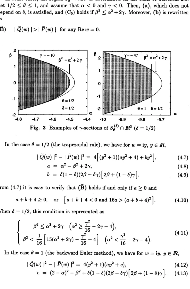
$\square$

(10)

In

some

cases, the region $S_{\theta}^{(\delta)}\cap R^{3}$ is determined

on

the basis of Theorem 2.1.

Let

$1/2\leq\theta\leq 1$,

and

assume

that

$\alpha<0$

and

$\gamma<0$

.

Then, (a),

which does

not

depend

on

$\delta$, is satisfied, and $(\mathrm{C}_{0})$ holds if$\beta^{2}\leq\alpha^{2}+27$. Moreover, (b) is rewritten

as

(B) $|\tilde{Q}(w)|>|\tilde{P}(w)|$ for any ${\rm Re} w=0$

.

Fig. 3Examples of $\gamma$-sections of $S_{\theta}^{(\delta)}\cap R^{3}(\delta=1/2)$

In the

case

$\theta=1/2$ (the trapezoidal rule),

we

have for

w

$=\mathrm{i}y$, y $\in R$,

$|\tilde{Q}(w)|^{2}-|\tilde{P}(w)|^{2}=4[(y^{2}+1)(ay^{2}+4)+by^{2}]$, (4.7)

$a=\alpha^{2}-\beta^{2}+2\gamma$, (4.8)

$b=\delta(1-\delta)(2\beta-\delta\gamma)[2\beta+(1-\delta)\gamma]$

.

(4.9)

Prom (4.7) it is easy to verify that (B) holds if and only if a $\geq 0$ and

$a+b+4\geq 0$, or

$[a+b+4<0$

and 16a $>(a+b+4)^{2}]$

.

(4.10)

When $\delta$ $=1/2$, this condition is represented as

$\{$

$\beta^{2}\leq\alpha^{2}+2\gamma$ $( \alpha^{2}\geq\frac{\gamma^{2}}{16}-2\gamma-4)$,

$\beta^{2}<\frac{1}{16}[15(\alpha^{2}+2\gamma)-\frac{\gamma^{2}}{16}-4]$ $( \alpha^{2}<\frac{\gamma^{2}}{16}-2\gamma-4)$

.

(4.11)

In the

case

$\theta=1$ (the backward Euler method),

we

have for w $=\mathrm{i}y$, y $\in R$,

$|\tilde{Q}(w)|^{2}-|\tilde{P}(w)|^{2}=4(y^{2}+1)(ay^{2}+c)$_, _(4.12)

c $=(2-\alpha)^{2}-\beta^{2}+\delta(1-\delta)(2\beta-\delta\gamma)[2\beta+(1-\delta)\gamma]$

.

(4.13)

(11)

The condition

(B)

holds

if

and

only

if

a

$\geq 0$,

c

$>0$,

which is

equivalent

to

$\beta^{2}\leq\alpha^{2}+2\gamma$, $\alpha<\frac{\gamma}{4}+2$, (4.14)

when $\delta=1/2$

.

References

[1] V. K. Barwell, Special stability problems for functional differential equations,

BIT 15 (1975), 130-135.

[2] M. Calvo and T. Grande, On the asymptotic stability of $\theta$-methods for delay

differential equations, Numer. Math. 54 (1988),

257-269.

[3] N. Guglielmi, Delay dependent stability regions of $$-methods for delay

differ-ential equations, $IMA$ J. Numer. A$nal$. 18 (1998), 399-418.

[4] M. Z. Liu and M. N. Spijker, The stability of the $\theta$-methods in the numerical

solution ofdelaydifferentialequations, $IMA$ J. Numer. Anal., 10 (1990), 31-48.

[5] L.$\cdot \mathrm{H}$. Lu, Numerical stability of the $\theta$-methods forsystems ofdifferential

equa-tions with several delay terms, J. Comput. Appl. Math., 34 (1991), 291-304.

[6] K. J. in ’$\mathrm{t}$ Hout, The stability of $\theta$-methods for systems of delay differential

equations, Ann. Numer. Math. 1(1994), 323-334.

[7] T. Koto, Stability of Runge-Kutta methods for delay integr0-differential

equa-tions, to appear in J. Comput. Appl. Math.

[8] G. Polya and G. Szego, Problems and theorems in analysis $\mathrm{I}$, Springer-Verlag,

Berlin, 1972.

[9] E. G. van den Heuvel, Using resolvent conditions to obtainnew stability results

for $\theta$-methods for delay differentialequations, $IMA$ J. Numer. Anal., 21 (2001),

421-438.

[10] D. S. Watanabe and M. G. Roth, The stability of difference formulas for delay

differential equations, SIAM J. Numer. Anal., 22 (1985), 132-145.

[11] M. Zennaro, $\mathrm{P}$-stability properties of Runge-Kutta methods for delay

differen-tial equations, Numer. Math., 49 (1986), 305-318.

[12] M. Zennaro, Delay differential equations: theory and numerics, in M.

Ainsworth, J. Levesley, W. A. Light, M. Marietta (ed.), “Theory and Numerics

ofOrdinary and Partial Differential Equations”, , Oxford University Press, New

York, 1995, 291-333.

[13] B. Zubik-Kowal, Stability in the numerical solution of linear parabolic equations

with adelay term, BIT41 (2001), 191-206