How Many Firms Should Be Leaders? Beneficial
Concentration Revisited
journal or
publication title
Discussion paper series
number
48
page range
1-37
year
2009-10
DISCUSSION PAPER SERIES
Discussion paper No.48
How Many Firms Should Be Leaders?
Beneficial Concentration Revisited
Hiroaki Ino
School of Economics, Kwansei Gakuin University and
Toshihiro Matsumura
Institute of Social Science, University of Tokyo
October, 2009
SCHOOL OF ECONOMICS
KWANSEI GAKUIN UNIVERSITY
1-155 Uegahara Ichiban-choHow Many Firms Should Be Leaders?
Beneficial Concentration Revisited
Hiroaki Ino∗
School of Economics, Kwansei Gakuin University and
Toshihiro Matsumura†
Institute of Social Science, University of Tokyo
Abstract
We investigate the relationship between the Herfindahl-Hirschman Index (HHI) and welfare. First, we discuss the model wherein m leaders and N − m followers compete. Daughety (1990) finds that under linear demand and constant marginal cost, the Stackelberg model yields larger welfare and HHI than the Cournot model. Thus, he demonstrates that beneficial concentration occurs. We find that this always occurs under general cost and demand functions when m is sufficiently large, but does not always occur when m is small. Next, we consider the free entry of followers, and find that beneficial concentration always occurs regardless of m. In particular, the more persistent the leadership, the more likely it is to be beneficial.
JEL classification numbers: L13, L40
Key words: HHI, beneficial concentration, leadership, free entry market
∗Corresponding author. Address: 1-155 Uegahara Ichiban-cho, Nishinomiya, Hyogo 662-8501, Japan. E-mail:
1
Introduction
Market concentration, measured by the Herfindahl-Hirschman Index (HHI), has played a rather important role in the context of antitrust legislations and economic regulations and it is increasingly gaining importance.1 For many years, HHI has also received considerable attention from researchers in a wide range of fields, including both economists and law scholars.
Market concentration and economic welfare are affected by both the number of firms and the asymmetries among the firms. The effect of the number of firms is usually straightforward. Typ-ically, in symmetric equilibria, an increase in the number of firms improves economic welfare and reduces the HHI.2 In contrast, the effect of the asymmetries among the firms is complex. Daughety (1990) investigates this problem by considering asymmetric roles among the firms. He formulates a model where m Stackelberg leaders and N − m Stackelberg followers compete in a homogeneous good market and discusses the relationship between m and economic welfare. Using a linear demand function and constant marginal cost, he finds an inverse U-shaped relationship between m and eco-nomic welfare. He demonstrates that the Stackelberg model (m ∈ (0, N )) yields larger welfare and HHI as compared to the Cournot model (m = 0 or m = N ). The heterogeneity of the roles among the firms increases HHI and at the same time, improves welfare (beneficial concentration).
In this paper, we examine this problem closely. We extend Daughety’s model in two directions. First, we consider general demand and cost functions. In particular, the generalization of the cost function is important since under strictly convex cost, asymmetric roles among the firms give rise to the production inefficiency, which does not arise under linear cost; hence, it is unclear whether beneficial concentration occurs. We find that given the total number of firms N , the introduction of a small number of followers into the Cournot model–implying that m decreases slightly from N –as in Daughety, always improves welfare and increases HHI. This result is robust because it holds
1For example, the Fair Trade Commission in Japan finally published a merger guideline based on the HHI in 2003,
although it denied using the HHI for many years.
2If we consider economies of scale, a large number of firms can be harmful. See, e.g., Mankiw and Whinston (1986)
true under general cost and demand functions. The result indicates that beneficial concentration can occur even under general demand and cost functions. On the other hand, we find that the introduction of a small number of leaders into the Cournot model–implying that m increases slightly from 0–also increases HHI but does not always improve welfare. Such an introduction can yield smaller welfare and higher HHI. Of course, if the marginal cost is constant, the introduction of a small number of leaders into the Cournot model always improves welfare and increases HHI (beneficial concentration). However, the latter result is not robust and does not hold true under increasing marginal cost. Thus, the relationship between HHI and economic welfare becomes much more complex when marginal cost is increasing.
Next, we endogenize the number of followers by considering the free entry of followers.3 We consider two types of long-run models that are different with respect to the persistence of leadership. In the first model (model 1), the production commitment by the leaders does not hold longer than the entry decision of followers; in the second model (model 2), it holds longer. In contrast to the case where the number of firms is exogenous, in both models 1 and 2, we find that the existence of leaders always improves welfare regardless of the number of leaders m. In other words, beneficial concentration caused by the heterogeneous roles among the firms always occurs in free-entry markets. This result indicates that HHI might be less appropriate for the measurement of welfare in free-entry markets as compared to markets with high entry barriers. It is also shown that model 2 yields larger welfare than model 1 for any m. This indicates that the more persistent the leadership, the more likely it is to be beneficial for welfare.
Finally, we discuss the properties of optimal states in a short-run model and two long-run models where m is adjusted to attain the highest welfare. We find that while the market with some leaders
3For the Stackelberg model with endogenous entry of firms, Etro (2006, 2008) also considers the model with free
entry of followers. His model has a single leader and the time structure is as in our model 2. For an application of the Stackelberg model with free entry of followers to the innovation, see Etro (2004). For the limit result when the number of followers entering goes to infinity, see Ino and Kawamori (2009). For the implications of public policy in free entry markets, see Davidson and Mukherjee (2007), Brand˜ao and Castro (2007), Mukherjee and Mukherjee (2008), and Marjit and Mukherjee (2008).
and some followers is optimal in the short-run model and long-run model 1, the market where all the followers’ entries are deterred by the leaders is optimal in long-run model 2. This result provides an important implication for deregulation policies. When a regulated market is converted into a free-entry one, the non-existence of new firms’ entries is often regarded as a bad signal and is associated with the leading incumbents’ abuse of market power, which results in entry barriers. However, surprisingly, according to the above results, this situation can be desirable if such a leadership is sustained for very long.
The paper is organized as follows. Section 2 formulates the model where the number of firms is exogenous (short-run model). Section 3 investigates the equilibrium outcomes and presents the results in a general setting; further, Section 3 specifies the demand and cost functions and provides an insightful example. Section 4 extends the model into the two models with free entry of followers (long-run models) and compares each with the Cournot case and also compares the two models themselves. Section 5 discusses the properties of the optimal number of firms. Section 6 briefly examines the integer problem related to the number of firms. Section 7 concludes the paper and provides some insights about heterogeneity of technologies and strategic complementarity for future researches. The proofs for the Lemmas and Propositions are presented in the Appendix.
2
Model
We formulate an N -firm oligopoly (N > 0). Firms produce a homogeneous product with identical cost function C(x) + f , where C(x) : R+ 7→ R+ is the production cost and f (≥ 0) is the fixed entry cost. The (inverse) demand function is given by P (X) : R+ 7→ R+. Each firm’s payoff is its own profit. Firm i’s profit πi is given by P (X)xi− C(xi) − f , where xi is firm i’s output and
X ≡PNi=1xi.
We make the following standard assumptions.
Assumption 1. P (X) is twice differentiable and P0(X) < 0 for all X such that P (X) > 0.
Assumption 3. P00(X)x + P0(X) < 0 for all X such that P (X) > 0 for all x ∈ (0, X).
Assumption 3 ensures that each firm’s marginal revenue is decreasing in the rivals’ outputs and that the reaction curve in the Cournot model has a negative slope, that is, the firms’ strategies are strategic substitute.
The game runs as follows. In the first stage, m(∈ [0, N ]) firms (Stackelberg leaders) inde-pendently choose their outputs. In the second stage, n (≡ N − m) firms (Stackelberg followers) independently choose their outputs after observing the leaders’ outputs.4 This model corresponds to the Cournot model when m = 0 or m = N .
We call the subgame perfect equilibrium symmetric if all leaders (followers) choose the same output level. The leaders’ output is of course different from that of the followers even in a symmetric equilibrium. We make an assumption on the equilibrium outcomes.5
Assumption 4. The model has a unique equilibrium for all m ∈ [0, N ]. The equilibrium is symmetric, and all firms produce positive outputs.
Finally, social welfare W (consumer surplus plus the profits of all the firms) is defined as W = Z X 0 P (q)dq − N X i=1 (C(xi) + f ). (1)
HHI is defined as the sum of the square of each firm’s market share: HHI ≡ N X i=1 ³ xi X ´2 .
3
Short-run analysis
In this section, we analyze the relationship between m and social welfare under the short-run case where N is exogenous.
4Here, we ignore the integer problem of the number of firms to grasp the essential properties of the Stackelberg
model with multiple leaders or free entry of followers. We discuss this integer problem in section 6.
5Sherali (1984) provides a sufficient condition for the existence of a unique equilibrium in a model with multiple
The solution (x∗
L(m), x∗F(m)) of the following system of equations corresponds to the equilibrium
outputs of leaders and followers.6 Note that (2) and (3) are the first-order conditions for leaders and followers, respectively.
(1 + nR0(XL∗))P0(X∗)x∗L+ P (X∗) − C0(x∗L) = 0, (2) P0(X∗)x∗F + P (X∗) − C0(x∗F) = 0, (3) where the equilibrium aggregate output X∗(m) = mx∗L(m) + nx∗F(m) and the equilibrium aggregate outputs of leaders X∗
L(m) = mx∗L(m). R(XL) represents each follower’s reaction to the leaders’ total
output XL.7 R(X
L) is obtained from the follower’s first-order condition and is given by
P0(XL+ nR(XL))R(XL) + P (XL+ nR(XL)) − C0(R(XL)) = 0. (4) Differentiating the above yields
R0(XL) = − P0(XL+ nR) + P00(XL+ nR)R
n(P0(XL+ nR) + P00(XL+ nR)R) + (P0(XL+ nR) − c00(R)). (5)
From Assumptions 1–3, we obtain nR0(X
L) ∈ (−1, 0) when m ∈ [0, N ). This implies that an
increase in the leaders’ output leads to a decrease in the followers’ output; the total output of all firms (including the leaders and the followers), however, increases.
By substituting the equilibrium outcomes into (1), we obtain the equilibrium social welfare W∗:
W∗(m) = Z X∗
0
P (q)dq − mC(x∗L) − nC(x∗F) − N f. (6) Further, let the equilibrium profit of a leader be given by π∗
L(m) = P (X∗(m))x∗L(m) − C(x∗L(m))
and that of a follower be given by π∗
F(m) = P (X∗(m))x∗F(m) − C(x∗F(m)).
6More precisely, the correspondence between (x∗
L(m), x∗F(m)) and equilibrium output is as follows. When m ∈
(0, N ), x∗
L(m) represents a leader’s equilibrium output and x∗F(m) represents a follower’s (the Stackelberg model).
When m = 0 and m = N , (3) and (2) respectively correspond to the first-order condition of the Cournot model with
N firms. Thus, xF(0) = xL(N ) is the equilibrium output of each firm when N firms produce simultaneously (the
Cournot model). Furthermore, although (2) ((3)) has no economic implications when m = 0 (m = N ), we can solve this equation and obtain xL(0) (xF(N )). Although Assumption 4 does not directly guarantee that (2) ((3)) has the
solution when m = 0 (m = N ), we can show that xL(0) (xF(N )) is well defined from Assumptions 1–4.
7From Assumptions 1–3, we can show that all subgames in the second stage have a unique equilibrium and that it
3.1 Welfare comparison
Let subscript ‘C’ denote the equilibrium outcomes when N firms produce simultaneously (the Cournot model). We present a result highlighting the difference between the Cournot outcome (where m = 0 or m = N ) and Stackelberg outcome (where m ∈ (0, N )).
Lemma 1 Suppose that Assumptions 1–4 are satisfied. Then, for all m ∈ (0, N ), (i) x∗
L(m) > x∗C,
(ii) x∗
F(m) < x∗C and (iii) X∗(m) > XC∗.
We present the results pertaining to the relationship between m and welfare. Proposition 1 focuses on the case of constant marginal costs.
Proposition 1 Suppose that Assumptions 1–4 are satisfied. If C00(x) = 0 for all x ≥ 0 (i.e.,
constant marginal cost), then W∗(m) > W∗(0) for all m ∈ (0, N ).
As seen in Lemma 1(iii), Stackelberg leaders increase the aggregate output. As such, total benefit increases and approaches the level observed in a competitive market; this results in higher welfare. Daughety (1990) has already demonstrated this result under the assumptions of linear demand and constant marginal cost. Various concentration measures, such as HHI, increase when the market structure changes from Cournot to Stackelberg. In other words, Stackelberg-type competition results in market concentration. In contrast to the traditional belief, concentration does enhance welfare. Daughety refers to this as ‘beneficial concentration’.
We discuss the robustness of Proposition 1 by considering increasing marginal cost. Proposition 1 implies that the Stackelberg model always yields greater welfare than the Cournot model regardless of m. Proposition 2 states that this result is true when m is sufficiently large, whereas it does not hold when m is sufficiently small.
Proposition 2 Suppose that Assumptions 1–4 are satisfied. Then, (i) we can have ∂W∂m∗¯¯m=0 < 0 and (ii) we always have ∂W∗
∂m
¯ ¯
Proposition 2(i) indicates that Proposition 1–the Stackelberg model always brings higher welfare than the Cournot model–is not robust when marginal cost is increasing. Suppose that some leaders are introduced into the Cournot model. Then, as in the case of constant marginal costs, this increases the total output. This competition acceleration effect in turn improves welfare. On the other hand, each leader’s output is strictly larger than each follower’s. Since the marginal cost is increasing, total production cost is minimized when all firms produce the same output. Thus, the introduction of a small number of leaders reduces production efficiency. Stackelberg model can bring lower welfare than the Cournot model since the latter’s welfare-reducing effect can dominate the former’s welfare-improving effect;8 note that the welfare-reducing effect does not exist when marginal cost is constant.
Further, while Proposition 2(i) states that the introduction of a small number of leaders into the Cournot model can reduce welfare, Proposition 2(ii) indicates that the introduction of a small number of followers always improves welfare9. To explain the reasoning behind this contrast, we present a supplementary result.
Lemma 2 Suppose that Assumptions 1–4 are satisfied. Then, (i) x∗
C = x∗L(N ) = limm→Nx∗L(m) = limm→Nx∗F(m) = x∗F(N ),
and (ii) x∗
L(0) = limm→0x∗L(m) > limm→0x∗F(m) = x∗F(0) = x∗C.
The outputs of the Stackelberg leaders and followers converge to the Cournot output when m is close to N , whereas the leaders’ output does not converge to the Cournot output (while the followers’ output does) when m is close to 0.
When m = N , there are no followers. Thus, the leaders do not exhibit strategic behavior against other firms. The introduction of a small number of followers into the Cournot model compels the
8Similar trade-offs of two abovementioned effects are discussed in many contexts. See, among others, Lahiri and
Ono (1988, 1998) and Matsumura (1998, 2003).
9Note that ‘introducing a small number of followers’ implies that m decrease slightly from N . Needless to say,
∂W∗/∂m|
m=Nrepresents how W∗moves when m increase slightly from N . Thus, the introduction of a small number
of followers enhances welfare if the sign of ∂W∗/∂m|
leaders to exhibit strategic behavior. However, the number of leaders is large, whereas that of followers is small. Thus, the strategic effect is small, and each leader’s output increases slightly. This is why x∗
L(m) tends to x∗C when m tends to N . The same principle is not applicable when
m tends to 0. The introduction of a small number of leaders into the Cournot model compels the leaders to exhibit strategic behavior. Since the number of leaders is small and the number of followers is large, the strategic effect is significant on each leader’s output, resulting in a non-negligible difference between x∗L(m) and x∗C. This is why x∗L(m) does not converge to x∗C when m is close to 0.
We will now explain the rationale behind the contrast in Proposition 2. We explain why the introduction of a small number of followers into the Cournot model always improves welfare, whereas that the introduction of a small number of leaders can both reduce and improve welfare.
The following decomposition helps to explain Proposition 2(i): ∂W∗ ∂m ¯ ¯ ¯ m=0 = [π ∗ L(0) − πF∗(0)] + N [P (X∗(0)) − C0(x∗F(0))] ∂x∗ F ∂m ¯ ¯ ¯ m=0. (7)
The change in welfare by the introduction of small number of leaders is decomposed into two parts. First, the unit firm’s marginal change into a leader directly contributes to a renewal of its own profit (the first term). Lemma 2(ii) implies that this effect is positive, that is, the leadership enhances the welfare if we focus on the firm that becomes a leader. However, the new leader steals other firms’ business (the second term). In other words, the introduction indirectly results in the reduction of the other firms’ (followers’) outputs; this is harmful for welfare. The change in welfare depends on the relative size of these two effects.
On the other hand, Proposition 2(ii) is elucidated by the decomposition below. ∂W∗ ∂m ¯ ¯ ¯ m=N = [π ∗ L(N ) − π∗F(N )] + N [P (X∗(N )) − C0(x∗L(N ))] ∂x∗ L ∂m ¯ ¯ ¯ m=N. (8)
Similarly, the change in welfare by the introduction of a small number of followers is decomposed into two parts. In contrast to the previous case, Lemma 2(i), here, implies that the first effect
of the renewal (the first term) converges to zero, that is, the reduction in the profit of the firm that becomes a follower is insignificant. Therefore, the indirect effect of the introduction on the other firms (the second term) alone determines the change in welfare. In this case, this effect is business augmenting10. In other words, the change in the role a firm from a leader to a follower indirectly causes all the other firms, as leaders, to expand their outputs; this is beneficial for welfare. Therefore, welfare always increases.
Propositions 1 and 2(ii) imply the following:
Corollary 1 Suppose that Assumptions 1–4 are satisfied. Then, there exists m ∈ (0, N ) such that W∗(m) > W∗
C.
Since the introduction of a small number of followers into the Cournot model increases HHI, this corollary implies that beneficial concentration can occur under general cost and demand functions (note that HHI is minimized when m = 0 and m = N since there is no asymmetry in these cases). However, the introduction of a small number of leaders into the Cournot model does not always result in beneficial concentration since it increases HHI but can reduce welfare. In the next subsection, we demonstrate this by using linear demand and quadratic cost functions.
3.2 Linear demand and Quadratic cost
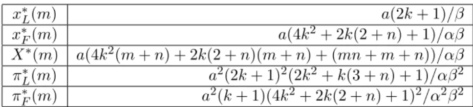
In this subsection, we specify the demand and cost functions and further elaborate on the relation between welfare and the number of leaders. Suppose that the inverse demand function is linear, i.e., P (X) = a − X, and the cost function is quadratic, i.e., C(x) = kx2, where k ≥ 0. Note that if k = 0 (k > 0), we have constant (increasing) marginal cost. The results obtained solving the model under these specifications (linear demand and quadratic cost), are summarized in Table 1, where n ≡ N − m. We can compute equilibrium social welfare in this specific case by substituting the results of Table 1 into
W∗(m) = 1 2(X
∗(m))2+ mπ∗
L(m) + nπF∗(m). (9)
x∗ L(m) a(2k + 1)/β x∗F(m) a(4k2+ 2k(2 + n) + 1)/αβ X∗(m) a(4k2(m + n) + 2k(2 + n)(m + n) + (mn + m + n))/αβ π∗ L(m) a2(2k + 1)2(2k2+ k(3 + n) + 1)/αβ2 π∗ F(m) a2(k + 1)(4k2+ 2k(2 + n) + 1)2/α2β2
Table 1: Results under the linear demand and quadratic cost functions: α = (2k + n + 1), β = (4k2+ 2k(2 + m + n) + (1 + m)) and n = N − m.
We demonstrate that leadership can reduce welfare under increasing marginal costs if the number of firms is sufficiently large.
Proposition 3 Assume linear demand and quadratic cost. If k > 0, there exists N0 > 0 such that ∂W∗
∂m
¯ ¯
m=0Q 0 if and only if N R N0.
Propositions 1 and 3 imply the following:
Corollary 2 Assume linear demand and quadratic cost. There exists N > 0 and m ∈ (0, N ) such that W∗(m) < W∗
C if and only if k > 0.
As discussed above, the introduction of leaders into the Cournot model always increases HHI. This corollary implies that the introduction of leaders into the Cournot model can reduce welfare, which is the traditional belief on market concentration. We present a numerical example for such a situation.
Numerical Example
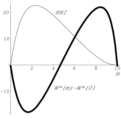
Suppose that a = 100, k = 0.2, f = 100 and N = 10. Using (9), we simulate how the ratio of leaders in the industry affects social welfare. Table 2 and Figure 1 depict a change in welfare when m changes in [0, 10] given N = m + n = 10. Compared to the Cournot case, as predicted in Proposition 3, the welfare is smaller when the ratio of leaders is small, while as predicted in Proposition 2(ii), the welfare is larger when the ratio of leaders is large. From Table 2, we can find that the welfare is maximum at m = 8.
m 1 2 3 4 5 6 7 8 9 W∗(m)/W∗(0) − 1 -0.41% -0.45% -0.33% -0.13% 0.08% 0.28% 0.46% 0.58% 0.55%
Table 2: Welfare increment by leadership in short run
Figure 1 also depicts how HHI reacts to the changes in the ratio of leaders. From this figure, we find that in our example, HHI provides a good insight into the change in welfare, except for when m tends to N . A decrease (increase) in HHI increases (decreases) welfare. In the case of constant marginal cost that Daughety (1990) investigates, the range in which both HHI and welfare increase is much wider. Under increasing marginal cost, however, an increase in concentration is more likely to be harmful, and this in turn is more likely to hold true when the number of leaders is small. Thus, it is reasonable that antitrust departments focus on markets with a small number of leaders.
************************************** Insert Figure 1 here.
**************************************
4
Free entry of followers
In this section, we consider the free entry of followers. We provide long-run cases where the existence of leaders always enhances social welfare even if the cost function is strictly convex. In other words, beneficial concentration always occurs when we introduce leaders into the Cournot model, even when marginal cost is increasing. We construct two models. In both models, the number of leaders m is given exogenously11while the number of followers n is determined endogenously.
The two models are distinguished by their time structures. In model 1, potential entrants (followers) decide whether to enter the market in the first stage. Then, all firms observe m and n. In the second stage, the m leaders choose their outputs. In the third stage, the n followers (n is
11If we consider the free entry of leaders, that is, if the number of leaders is endogenous and is determined by the
zero-profit condition, the followers obtain negative profits and thus, no follower enters the market. In other words, the equilibrium becomes the long-run Cournot equilibrium.
determined endogenously in the first stage) choose their outputs after observing the leaders’ output. In model 2, the m leaders choose their outputs in the first stage. In the second stage followers decide whether to enter the market. In the third stage, followers choose their outputs after observing n and the leaders’ outputs.
We provide some cases rationalizing each model.12 The key difference in these two models is the time at which the followers enter, that is, the relative flexibility of the followers’ entry choices to leaders’ production choices. Consider model 1. Suppose that m firms have a special ability to produce faster than the other firms.13 In other words, m firms can commit their production by inventory control and become leaders. Usually, inventory control does not increase the duration of production commitment compared to the entry decision. Thus, in this case, the leaders’ production follows the followers’ entry. Consider model 2. Suppose that m firms are incumbents and can make a certain capacity before the other firms. In other words, m firms can commit to their output level by capacity investments and become leaders. Usually, capacity investments can result in a production commitment before the entries of followers. Thus, in this case, the new entrants enter the market after the leaders have satisfied their production commitment. As a result, the new entrants become followers.
Henceforth, we assume the following to ensure that our long-run analysis is meaningful.
Assumption 5. Each long-run model has a unique equilibrium. The equilibrium number of followers is positive.
Note that this assumption implies that f > 0. Thus, the average cost (C(x) + f )/x follows a U-shaped pattern if the output minimizing average cost exists and is monotonically decreasing if the
12Other than the cases mentioned below, we can consider a wide variety of situations suitable for our long-run
models. For instance, production alliance, R&D facility, long-term contracts with customers, or sophisticated sales networks would give firms asymmetric rolls in an industry. The validity duration of commitments yielded in these ways depends on their frameworks and the environment of the industry. Thus, which model 1 or 2 is suitable is determined on a case-by-case basis.
13Some readers may think that such a special skill not only results in the emergence of the leadership but also
often enhances technology. However, our long-run analysis indicates that even if the effect on technology is neglected, beneficial concentration occurs.
output minimizing average cost does not exist.14
In the following two subsections, we demonstrate that the two models have similar implications on beneficial concentration.
4.1 Model 1: Followers’ entry before Stackelberg competition
In this subsection, we investigate model 1. Let n1(m) be the equilibrium number of followers, which is obtained from the following zero-profit condition for followers:
P (X1(m))x1F(m) − C(x1F(m)) − f = 0, (10) where X1(m) = mx1
L(m) + n1(m)x1F(m), and x1L(m) and x1F(m) represent the long-run equilibrium
output of a leader and a follower, respectively. N1(m) represents the total number of firms and is given by N1(m) = m + n1(m). Since the subgames following the followers’ entry decisions are the same as in the short-run model analyzed in Section 3, these equilibrium outcomes are obtained by conditions (2), (3) and (10). Using the expressions in the previous section, we have x1
L(m) = x∗L(m)
and x1
F(m) = x∗F(m) for N = N1(m). The case where m = 0 corresponds to the long-run Cournot
model (Cournot model with free entry). As in the previous sections, subscript C denotes the equilibrium outcome in the Cournot model.
We provide the relationship between the equilibrium outcomes of the Cournot and Stackelberg models.
Lemma 3 Suppose that Assumptions 1–5 are satisfied. Then, ∀m > 0, (i) x1
F(m) = x1C, (ii)
X1(m) = X1
C, (iii) x1L(m) > x1C and (iv) N1(m) < NC1.
Lemma 3(i) implies that each follower’s output does not depends on m. Since the equilibrium price is equal to the follower’s average cost (zero-profit condition), the equilibrium price remains
14If the average cost is decreasing (including the case of constant marginal cost with some fixed cost), Assumption 5
is never satisfied in model 2 (while it can be satisfied in model 1). This is because the aggregate output of the leaders undercuts the Cournot price in model 2, and no follower can enter in equilibrium. However, even in this case, if the given number of leaders is not wastefully large, beneficial concentration occurs since the optimal case with decreasing average cost is monopoly.
unchanged unless the follower’s output changes (this implies Lemma 3(ii)).
Lemma 3(i) is a key result. Regardless of m, the average cost curve of each follower must be tangent to the “residual demand curve” of each follower at the long-run equilibrium. As is easily guessed, the change from the Stackelberg model (m > 0) to the Cournot model (m = 0) reduces the leaders’ output for given n. This leads to an upward shift in each follower’s residual demand curve; however, in the long-run, it induces new entries, leading to a downward shift in each follower’s residual demand curve. Eventually, the upward shift of the residual demand curve is negated by the new entries, resulting in an unchanged curve. This is why the two models yield the same equilibrium output for each follower at the long-run equilibrium (see Figure 2).
************************************** Insert Figure 2 here.
**************************************
Let W1(m) denote the long-run equilibrium welfare for given m. Note that W1
C = W1(0) is the
equilibrium welfare in the Cournot-type model. Proposition 4 indicates a striking contrast to the short-run case.
Proposition 4 Suppose that Assumptions 1–5 are satisfied. Then W1(m) > W1
C ∀m > 0.
The introduction of a leader yields asymmetry among firms and increases HHI. In addition, it reduces the total number of firms (Lemma 3(iv)), again leading to an increase in HHI. However, it improves welfare (Proposition 4). In other words, beneficial concentration always occurs.15 Notice that as seen in Lemma 3 (ii), since consumer surpluses are the same in both Cournot and Stackelberg equilibria, beneficial concentration occurs owing to the extra profit of the leaders. Thus, in this context, it is also inappropriate to uncritically use the extra profit of particular leading firms as a dangerous sign indicating monopoly power.
15Long- and short-run analysis often have different implications in oligopoly models. See, among others, Lahiri and
We explain the reasoning behind this result. Consider that some firms in the Cournot model become leaders. Recall that in the short-run case discussed in the previous section, the introduction of leaders yields the competition acceleration (welfare-improving effect) and production inefficiency (welfare-reducing effect). The relative size of these effects determines the total impact on welfare. In the long-run case, no competition acceleration effect arises since the number of leaders does not affect total output and price (Lemma 3 (ii)). Hence, the effect that needs to be discussed pertains to production efficiency. With regard to production efficiency, intuitively speaking, leaders’ aggressive behavior deters some followers from excessively entering16 and saves on the fixed cost. Why is it that this saving always dominates the production inefficiency arising from the asymmetry between leaders and followers? Lemma 3 shows that leaders’ total output increases and that followers’ total output decreases by the same amount. Since the increase in leaders’ total output is caused by the expansion of each firm’s output (Lemma 3(iii)), this production substitution approximately increases the leaders’ cost by C0(x
L) (leaders’ marginal cost) for every unit of output expansion. On the other
hand, the decrease in followers’ total output is because the number of followers entering is reduced; each follower’s output is constant (Lemmas 3(i) and 3(iv)). Thus, the production substitution reduces the followers’ cost by (C(xF) + f )/xF (followers’ average cost) for every unit of output reduction. Since followers’ average cost is equal to the price and leaders’ marginal cost is lower than the price,17each marginal unit of production substitution saves on cost. Therefore, in the long run, production substitution always improves production efficiency. Hence, the Stackelberg model always yields larger welfare than the Cournot model.
4.2 Model 2: Leadership before followers’ entry
In this subsection, we formulate a model with an alternative time structure. After observing the leaders’ outputs, new entrants decide whether or not to enter the market. Let superscript “2” denote the equilibrium outcomes in this model. Note that even in this model, m = 0 corresponds
16As for the excess entry, see Mankiw and Whinston (1986) and Suzumura and Kiyono (1987). 17Note that by Lemma 3(ii), the price is common for the Cournot and Stackelberg models.
to the long-run Cournot model. Therefore, we have x2
C = x1C, XC2 = XC1 and NC2 = NC1 (subscript
C denotes the outcomes in the Cournot model).
Lemma 4 Suppose that Assumptions 1–5 are satisfied. Then, ∀m > 0, (i) x2
F(m) = x2C, (ii)
X2(m) = X2
C, (iii) x2L(m) > x2C and (iv) N2(m) < NC2.
Lemma 4 is similar to Lemma 3, indicating that the results derived in model 1 also holds true in model 2.
Fundamentally, models 2 and 1 differ only in terms of the followers’ reactions to the leaders’ actions. In model 2, when the followers react to the leaders’ output levels, the former may not only change their output levels but also take decisions pertaining to their entry/exit in the market. Therefore, at any given level of the leaders’ output, each follower’s output and thus, the total output are always equal to those in the Cournot model due to the same reason as in Lemma 3. Thus, the equilibrium price is constant regardless of the leaders’ actions. In other words, the leaders become price takers at the Cournot price. As a result, a leader’s output in this model exceeds that in the Cournot model.
Proposition 5 Suppose that Assumptions 1–5 are satisfied. Then, W2(m) > W2
C ∀m > 0.
The introduction of leaders increases HHI; this is as in the previous subsection. Therefore, Propo-sition 5 states that beneficial concentration always occurs in model 2 as well as in model 1. The proof and intuition for Proposition 5 are similar to that for Proposition 4; therefore, these have been excluded. Etro (2008) also shows that when m = 1, Stackelberg competition in model 2 yields higher welfare than Cournot competition with free entry.18 Thus, our result in Proposition 5 is an extension of his result for the model with multiple leaders.
4.3 Comparison of models 1 and 2
As seen in the previous two subsections, when the Stackelberg case is compared to the Cournot case, models 1 and 2 have a similar effect on beneficial concentration. However, these two models are distinct if we compare their equilibrium outcomes.
Lemma 5 Suppose that Assumptions 1–5 are satisfied. Then, ∀m > 0, (i) x1
F(m) = x2F(m), (ii)
X1(m) = X2(m), (iii) x1
L(m) < x2L(m), and (iv) N1(m) > N2(m).
Lemma 5 implies that each follower’s output and total output are the same in the two models. However, each leader’s output levels and the number of followers are different for the two models.
In model 2, the leaders behave as price takers at the Cournot price. On the other hand, in model 1, the leaders’ marginal cost is still lower than the Cournot price. Since the Cournot price is the same in both models, each leader’s equilibrium output is larger in model 2 than in model 1, and as a result, the number of followers is smaller in model 2 than in model 1. Since in model 2, leaders choose their outputs taking followers’ entry into consideration, they become more aggressive and as a result, more effectively deter followers from entering. Since the source of beneficial concentration is the savings in followers’ entry cost, it is straight-forward that model 2 yields higher welfare than model 1.
Proposition 6 Suppose that Assumptions 1–5 are satisfied. Then, W2(m) > W1(m) ∀m > 0. Proposition 6 states that the beneficial impact of long-run leadership on welfare is greater in model 2 than in model 1. This implies that leadership is more desirable if the leadership persistently adopts a more inflexible production position to followers’ entry choices.
Numerical Example
To illustrate the properties of the two long-run models in detail, we provide numerical results. Suppose linear demand P (X) = a − X and quadratic cost C(x) = kx2, where k ≥ 0. Further,
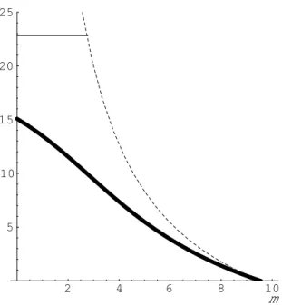
a = 100, k = 0.2, f = 100 (these parameters are the same as in the numerical example in Subsection 3.2). Figures 3, 4 and 5, respectively, depict how the long-run equilibrium output of a leader, number of followers and welfare change in m. From Lemma 5 and Proposition 6, we have x1
L(m) < x2L(m),
n1(m) > n2(m) and W2(m) > W1(m) as far as followers enter. Table 3 numerically expresses the welfare change. We find that m = 4 yields maximum welfare in model 1. On the other hand, in model 2, we can see that welfare is increasing in m. This observation provides us with a conjecture that there will be some differences between models 1 and 2 with regard to the reaction of welfare to the changes in the number of leaders. We will discuss this in the next section.
m 1 2 3 4 5 6 7 8 9
W1(m)/W1(0) − 1 2.28% 4.14% 5.39% 5.92% 5.79% 5.11% 4.02% 2.62% 0.98% W2(m)/W2(0) − 1 2.74% 5.48%
Table 3: Welfare and the number of leaders in the long run
************************************** Insert Figures 3–5 here.
**************************************
5
Optimal number of leaders
In this section, we discuss the properties of the optimal number of leaders in the short-run model and the two long-run models.
Proposition 7 Suppose that Assumptions 1-4 are satisfied. (i) In the short run, the number of leaders that yields the maximum W∗(m) is in (0, N ). Suppose, in addition, that Assumption 5 is
satisfied. (ii) In the first long-run model (model 1), the number of leaders that yields the maximum W1(m) is in (0, NC1). (iii) In the second long-run model (model 2), W2(m) is increasing in the number of leaders.
Both (i) and (ii) state that the market with both leaders and followers is desirable. However, with regard to (i), as seen in Figure 1, we can state that the equilibrium welfare when the number of leaders is small can be less than that in the Cournot case (rotated S-shaped relationship between m and W∗(m) in Figure 1). On the other hand, with regard to (ii), as seen in Figure 5, the equilibrium
welfare for any given number of leaders is greater than that in the Cournot case (inverse U-shaped relationship between m and W1(m) in Figure 5). Therefore, while the optimal number of leaders in model 1 is typically not that large (somewhere around NC1/2), the optimal number of leaders in the short-run model tends to be large (biased towards N ).19
There is a sharp contrast in (ii) and (iii). While the optimal number of leaders in model 1 is such that some followers are allowed to enter, the number of leaders in model 2 is, as long as some follower enters (Assumption 5), more desired if it gets larger. This implies that the optimal number of leaders in model 2 is such that no follower is allowed to enter, Indeed, if we relax Assumption 5 and include the case where no follower is allowed to enter, we obtain the optimal number of leaders for model 2.20
If we consider the constant marginal cost case, the second contrast is remarkable. As noted in Etro (2006), in Model 2 with constant marginal cost, single leader blocks all the followers from entering. Thus, this leader can earn huge profits by undercutting the long-run Cournot price. Welfare is enhanced by this amount; the savings made on followers’ fixed cost is substantially large. On the other hand, in Model 1 with the constant marginal cost, some followers enter the market as long as m < N1
C. Therefore, m ≥ NC1 must hold if the leaders are to block all the followers from
19Recall that in the simulations, the optimal number of leaders in m = 8 in the short-run model and m = 4 in
model 1.
20Consider the case where m is so large that x2
F(m) = 0 holds. When m ≥ NC2, the m-firms’ Cournot price is lower
than or equal to P (X2
C). Thus, we find that the equilibrium of model 2 is the Cournot equilibrium with m firms.
When m ≤ N2
C, the m-firms’ Cournot price is higher than or equal to P (XC2). Thus, the situation where each leader
produces X2
C/m is one of the equilibria of model 2 (the equilibrium price is P (XC2), and x2F(m) = 0). In this case,
the dotted line in Figure 5 (Figure 3) denotes the change in welfare (each leader’s output) in m. If m is larger than the point at which the dotted line tangent to the thin line, no followers enter. If m = N2
C which is the point at which
X2
C/m = x2Cholds, the situation corresponds to the m-firm Cournot equilibrium. Therefore, by Proposition 7(iii), the
optimal number of firms must be between these two points. Observe that in the figure, if we connect the thin line and the dotted line, the inverse U-shaped relationship between m and W2(m), which is greater than W1(m), emerges.
entering. Hence, there are no savings on fixed cost.
6
Integer problem
Finally, we provide some qualifications for our results on beneficial concentration with respect to an integer problem. Although our main results in Corollary 1, Proposition 4 and Proposition 5 suggest a tendency towards beneficial concentration, we have, thus far, not considered the integer constraint for the number of firms. Corollary 1 depends on the fact that we can slightly decrease the number of leaders, while Propositions 4 and 5 depend on the fact that the number of followers is a real number. Thus, it is important to consider the integer constraint.
However, in the short-run model, we obtain similar results even when there is an integer con-straint if the model has a linear demand and quadratic cost (as in Subsection 3.2). More concretely, we can show that under the constraint N ∈ {2, 3, · · · }, (i) when k > 0, there exists N0 > 2 such
that W∗(1) − W∗(0) ≶ 0 if and only if N ≷ N0 and (ii) W∗(N − 1) − W∗(N ) > 0 for all N .21 The integer problem is more serious in the long-run models. Suppose that the number of firms is an integer. Then, if not even only additional entry is profitable, the firms do not enter even when each follower makes a positive profit. This implies that the long-run price can exceed the followers’ average cost. Thus, the integer constraint reduces the consumer surplus. If the integer problem is more severe in the Stackelberg model than in the Cournot model, integer constraint works as a counter effect to the beneficial concentration. Indeed, in both models 1 and 2, we can present counter examples wherein the beneficial concentration does not occur for some m even in the model with linear demand and quadratic cost (shown in Appendix B).
7
Concluding remarks
In this paper, we analyze welfare in a model with multiple Stackelberg leaders and reexamine the relationship between HHI and welfare. We find that beneficial concentration always occurs when
a small number of followers are introduced. In contrast, the introduction of a small number of leaders can both reduce and improve welfare. Such an introduction, however, always increases HHI. We also find that if we consider the free entry of followers, beneficial concentration always occurs when we introduce a leader into the Cournot model. This result indicates that HHI might be less appropriate for the measurement of welfare in free-entry markets than in markets with high entry barriers. In particular, beneficial concentration always occurs even if the leaders do not take the entry of followers into account (model 1). However, if the leadership is so persistent that the leaders can take the entry of followers into account (model 2), it is more beneficial for welfare. Indeed, in this case, the optimal number of leaders is such that no follower is allowed to enter.
In long-run models, we assume that the number of leaders is given exogenously. This setting implies that a limited number of firms have the ability to become leaders. In reality, there are various situations that are suitable for this limited leadership, for example, incumbents with bottleneck facilities as in the power industry, long-established firms in a production alliance as in the airline industry and pioneering firms successfully creating brand loyalty among their consumers as in the mobile phone market.22 In antitrust policies, limited leadership is often considered as a problem that results in entry barriers. However, our result indicates that the possibility of preventing inefficient entries enhances welfare if the leadership is retained for a long time.
In this paper, we assume that all firms have identical cost functions and that only the difference of roles among the firms yields asymmetry. However, particularly in our long-run models, the reasoning behind Lemma 3(i) is applicable even if we introduce leaders whose cost is different from that of the entrants in the Cournot model. Hence, the price and followers’ profits remain unchanged after the introduction, and thus, the entire net social benefit of this introduction must serve as a reward for the leaders. Thus, we obtain the implications on welfare comparison: the welfare in the Stackelberg model (m > 0) is greater than that in the Cournot model (m = 0) if and only if
22See Etro (2007) for other examples and applications. In chapter 6, he argues that Microsoft in the software market
the profits of the leaders are positive. If we introduce the cost differences among firms into the short-run model, the analysis will become more complicated. Leadership by a firm with a lower (higher) marginal cost is more likely to improve (reduce) welfare. However, it is difficult to find another condition for welfare improvement since not only the leaders but also the followers and consumers are relevant to changes in welfare. Extending our analysis in this direction remains for future research.23
In the body of this paper, the key explanation of the welfare improvement was the aggressive behavior of the leaders. Thus, Assumption 3, which indicates that the firms’ strategies are strategic substitute, seems to be the critical assumption for the beneficial concentration. However, this will only be true in the short run and not necessarily true in the long run. In the games where the firms’ strategies are strategic complement, leadership makes the firms accommodative and thus, reduces the total output in the short run. This implies that the competition accelerating effect mentioned in the case of strategic substitute is replaced by the competition decelerating effect. At the same time, the production inefficiency caused by the asymmetric production between leaders and followers remains. Since leadership reduces welfare in both the aspects, welfare improvement does not occur in the short run. Let us consider the long-run time structure as in model 1 and the firms’ strategies as strategic complement. Then, the free entry in Cournot competition results in insufficient entries.24 If some firms assume leadership, their accommodative behavior will further increase the number of entries and this will alleviate the insufficiency of the entries and improve welfare. However, more formal and general analysis will be needed in this regard. This is left for the future.25
23For the discussion with a single leader and a fixed number of followers under cost heterogeneity, see Levin (1988).
For the discussion on endogenous roles among firms with heterogeneous costs, see Ono (1978,1982). For the discussion of the endogenous role of N-firm oligopoly, see Matsumura (1999) among others. For the discussion on the role of firms based on experimental studies, see Huck et al. (2001).
24See footnote 7 in Mankiw and Whinston (1986).
25For a time structure as in model 2, Etro (2008) provides the applications of price competition with Logit demand
APPENDIX
A
Proofs
Proof of Lemma 1: In Section 3, we have already shown that an increase (decrease) of xL
decreases (increases) xF and increases (decrease) X given m and n (see the discussion immediately
after equation (5)). Thus, Lemma 1(i) implies Lemma 1(ii) (Lemma 1(iii)) and vice versa. Thus, we merely have to prove Lemma 1(i). We prove it by contradiction. We assume x∗L(m) ≤ x∗C and derive a contradiction. Note that x∗
L(m) ≤ x∗C implies X∗(m) ≤ XC∗.
Substituting m = 0 into (3) yields
P0(XC∗)x∗C+ P (XC∗) − C0(x∗C) = 0, (11) where X∗
C = X∗(0) = N x∗C = N x∗F(0). We compare the LHS in (11) with that in (2). Assumption 3
ensures that P0(X)x + P (X) is decreasing in X. Since X∗(m) ≤ X∗
C, we have P0(XC∗)x∗C+ P (XC∗) −
C0(x∗
C) ≤ P0(X∗(m))x∗C + P (X∗(m)) − C0(x∗C). Since P0 < 0, C00 ≥ 0, and x∗L(m) ≤ x∗C, we have
P0(X∗(m))x∗C + P (X∗(m)) − C0(x∗C) ≤ P0(X∗(m))x∗L(m) + P (X∗(m)) − C0(x∗L(m)). As is shown in Section 3 (immediately after equation (5)), −1 < (N − m)R0 < 0 for m ∈ [0, N ). Thus we have P0(X∗(m))x∗
L(m) + P (X∗(m)) − C0(x∗L(m)) < (1 + (N − m)R0)P0(X∗(m))x∗L(m) + P (X∗(m)) −
C0(x∗
L(m)). Therefore, if (11) is satisfied, the LHS in (2) must be positive, a contradiction. Q.E.D.
Proof of Proposition 1: Let c denote the (constant) marginal cost. Then we obtain W∗(m) − W∗(0) =
Z X∗(m)
X∗ C
P (X)dX − c(X∗(m) − XC∗) > [P (X∗(m)) − c](X∗(m) − XC∗) > 0. The inequalities hold since the price exceeds the marginal cost and from Lemma 1(iii). Q.E.D. Proof of Proposition 2: (i) Proposition 3 in Section 4 presents examples where ∂W∂m∗¯¯m=0 < 0 when N > N0.
(ii) We show that for any situation satisfying Assumptions 1–4, ∂W∗(N )/∂m < 0.
Differenti-ating (6) and evaluDifferenti-ating at m = N , we obtain (8). Since x∗
L(N ) = x∗F(N ) = x∗C (Lemma 2(i)),
π∗
L(N ) − π∗F(N ) is canceled out. Thus, if the last term on the RHS of (8) is negative, ∂W∗/∂m|m=0
is also negative. Comparative statics analysis using (2) and (3) yields ∂x∗ L ∂m ¯ ¯ ¯ m=N = P0x∗ C(P0− C00(x∗C))R0|m=N N (P0+ P00x∗ C)(P0− C00(x∗C)) + (P0− C00(x∗C))2 < 0 (12) where R0|m=N = −(P0(XC∗) + P00(XC∗)x∗C)/(P0(XC∗) − C00(x∗C)) < 0. We use x∗L(N ) = x∗F(N ) = x∗C
to induce (12), which implies that the last term on the RHS is negative. Q.E.D. Proof of Lemma 2: We regard the LHS in (2) as a function F (m, x∗
L(m), x∗F(m)) and the LHS in (3) as a function G(m, x∗ L(m), x∗F(m)). Continuity of F (·) yields lim m→0F (m, x ∗ L(m), x∗F(m)) = F ³ 0, lim m→0(x ∗ L(m), x∗F(m)) ´ . On the other hand, since F (m, x∗
L(m), x∗F(m)) = 0 ∀m ∈ (0, N ), limm→0F (m, x∗L(m), x∗F(m)) = 0.
Hence, F (0, limm→0(x∗L(m), x∗F(m))) = 0. Similarly, G(0, limm→0(x∗L(m), x∗F(m))) = 0. Therefore,
limm→0(x∗L(m), x∗F(m)) is a solution of the system of equations (2) and (3) when m = 0. Thus, by
definitions of x∗
F(0), x∗L(0), and x∗C, we have limm→0x∗F(m) = x∗F(0) = x∗C and limm→0x∗L(m) =
x∗
L(0). Similarly, taking m → N , we obtain limm→Nx∗L(m) = x∗L(N ) = x∗C and limm→Nx∗F(m) =
x∗ F(N ).
Consider m = 0. Note that the proof of Lemma 1 is also applicable when m = 0. Therefore, x∗
L(0) > x∗C. Next, consider m = N . Note that when m = N , nR0 is canceled from (2). Thus,
x∗
L(N ) = x∗C is obtained only by (11). Then, given x∗L(N ) = x∗C, x∗F(N ) is determined according to
(3), i.e., P0(N x∗
C)x∗F + P (N x∗C) = C0(xF∗). x∗F(N ) satisfies this equation if x∗F(N ) = x∗C by (11).
Then, uniqueness of x∗F(N ) implies that x∗F(N ) = x∗C = x∗L(N ). Q.E.D.
results in table 1, we have
π∗L(0) = P (X∗(0))x∗L(0) − C(xL∗(0)) = (a − c)2(2k + b)2(2k2+ bk(3 + N ) + b2)
(2k + N b + b)(4k2+ 2bk(2 + N ) + b2)2 , (13) π∗F(0) = P (X∗(0))x∗F(0) − C(x∗F(0)) = (a − c)2(k + b)
(2k + N b + b)2. (14)
From the first-order condition (3),
P (X∗(0)) − C0(x∗F(0)) = −P0(X∗(0))x∗F(0) = bx∗F(0) = b(a − c) 2k + N b + b. (15) Differentiating x∗ F yields ∂x∗F ∂m ¯ ¯ ¯ m=0 = −N (a − c)b3 (2k + N b + b)2(4k2+ 2bk(2 + N ) + b2). (16) Substituting (13)–(16) into Equation (7), we obtain
∂W∗ ∂m ¯ ¯ ¯ m=0 = N (a − c)2b3A (2k + N b + b)3(4k2+ 2bk(2 + N ) + b2)2, (17) where A is given by A = [8k3+ 12k2b + 6kb2+ b3+ (2k2b + kb2)N ] − kb2N2.
Since the denominator is positive, the RHS of (17) is negative (positive) if and only if A < 0 (A > 0). Since k > 0, the first term of A, which is within the bracket, is positive, and the second term of A is nonpositive. Note that when N = 0, A > 0 because the second term is zero. The first term is linear and the second term is quadratic with respect to N . Hence, in absolute value, the second term must exceed the first term when N is greater than some positive number and vice versa. Q.E.D. Proof of Lemma 3: We prove that the firm facing the zero-profit condition produces on the downward-sloping part of the average cost curve. If the average cost is monotonically decreasing, this is obvious. Otherwise, let ˆx denote the output minimizing average cost of firm (C(x) + f )/x. We show that x1
F(m) ≤ ˆx. Suppose the contrary: x1F(m) > ˆx holds true. Consider that one follower
constant, the deviation reduces the total output, resulting in an increase in the price (note that the leaders have chosen their outputs before observing the followers’ outputs). Firm i’s profit is zero before the deviation from the zero profit condition (from (10)). The deviation increases the price and reduces firm i’s average cost and therefore, firm i makes a positive profit after the deviation. This is a contradiction. The same principle can be applied to the Cournot model to obtain x1
C ≤ ˆx.
(i) We prove x1
F(m) = x1C by contradiction. Suppose that x1F(m) < x1C. From (10) (zero profit
condition), we have P (X1(m)) = (C(x1
F) + f )/x1F and P (XC1) = (C(x1C) + f )/x1C. These equations
imply that P (X1(m)) > P (XC1) since the average cost (C(x) + f )/x is decreasing when x < ˆx and x1
F(m) < x1C ≤ ˆx by the supposition. Since P0 < 0, X1(m) < XC1 must hold. We compare the
LHS in (11) with that in (3). Assumption 3 ensures that under the condition X1(m) < X1
C, the
inequality P0(X1
C)x1C+ P (XC1) − C0(x1C) < P0(X1(m))x1C+ P (X1(m)) − C0(x1C) holds. Since P0< 0
and C00 ≥ 0, under the condition x1
F(m) < x1C, we have P0(X1(m))x1C + P (X1(m)) − C0(x1C) <
P0(X1(m))x1
F(m) + P (X1(m)) − C0(x1F(m)). Thus, if (11) is satisfied, the LHS in (3) must be
positive, which is a contradiction. Similarly, x1
F(m) > x1C leads to a contradiction.
(ii) From (10), we have P (X1(m)) = (C(x1
F) + f )/x1F and P (XC1) = (C(x1C) + f )/x1C. In Lemma
3(i), we have shown that x1
F(m) = x1C. Thus, P (X1(m)) = P (XC1). X1(m) = XC1 is derived from
P0 < 0.
(iii) Suppose the contrary, i.e., x1
L(m) ≤ x1C. We compare the LHS in (11) with that in (2). Since
P0 < 0 and C00 ≥ 0, under the condition x1
L(m) ≤ x1C, we have P0(XC1)x1C + P (XC1) − C0(x1C) ≤
P0(X1(m))x1L(m) + P (X1(m)) − C0(x1L(m)), where we use Lemma 3(ii). Since nR0(XL) ∈ (−1, 0)
(see the discussion immediately after equation (5)), P0(X1(m))x1L(m) + P (X1(m)) − C0(x1L(m)) < (1 + n1(m)R0)P0(X1(m))x1
L(m) + P (X1(m)) − C0(x1L(m)). Therefore, if (11) is satisfied, the LHS
in (2) must be positive, which is a contradiction.
Proof of Proposition 4: Lemma 3(ii) indicates that the consumer surplus in the Stackelberg model (m > 0) is equal to that in the Cournot model (m = 0). The profits of all firms in the Cournot model are zero by the zero profit condition (10). In the Stackelberg model, the profits of all followers are also zero. Since x1
L is larger than x1C by Lemma 3(iii) and is less than the output
level that equates the marginal cost with price by (2), the average cost of each leader (C(x1
L)+f )/x1L
is less than P (X1
C) = (C(x1C) + f )/x1C, which is equal to the equilibrium price in the Stackelberg
model. Therefore, the profits of all leaders are positive in the Stackelberg model. Q.E.D. Proof of Lemma 4: Let m > 0. Given the leaders’ aggregate outputs, the followers’ actions are determined according to the following equations (at the second stage and third stage).
P (X2(m))x2F(m) − C(x2F(m)) − f = 0, (18) P0(X2(m))x2F(m) + P (X2(m)) − C0(x2F(m)) = 0 (19) Since P (X2(m)) = P (X2
C) (from Lemma 4(ii)), a leader’s output (at the first stage) is obtained by
P (XC2(m)) = C0(x2L(m)). (20)
(i) Using these conditions, we can prove x2
F(m) = x2C in the same way as in the proof of Lemma
3(i). Note that in the proof of Lemma 3(i), (10), (3) and (11) are all the conditions to proove the fact. In this proof, (18) and (19) correspond to (10) and (3), respectively. The condition in Cournot model (11) is common in both models 1 and 2.
(ii) The proof is similar to that of Lemma 3(ii). (iii) In the Cournot model, P (X2
C) > C0(x2C). Thus, by (20) and C00 > 0, we have x2L(m) > x2C.
(iv) Lemma 3 (iv) is derived from Lemmas 3(i)–(iii). Q.E.D.
Proof of Lemma 5: (i) From Lemma 3(i) and Lemma 4(i), it is obvious that x1
F(m) = x1C =
x2
C = x2F(m).
(ii) Similarly, from Lemma 3(ii) and Lemma 4(ii), tt is obvious that X1(m) = X1
(iii) As seen in (2), x1
L(m) satisfies P (X1(m)) > C0(x1L(m)). As seen in (20), x2L(m) satisfies
P (X2(m)) = C0(x2
L(m)). Since from (ii), we have X1(m) = X2(m), C0(x2L(m)) > C0(x1L(m)) holds.
Therefore, we have x2
L(m) > x1L(m) from C00> 0.
(iv) Lemma 5(iv) is derived from Lemmas 5(i)–(iii). Q.E.D.
Proof of Proposition 6: Lemma 5(ii) indicates that the consumer surplus in model 1 is equal to that in model 2 for all m > 0. In both models 1 and 2, the profits of all the followers are zero. Observe that from (2) and (20), we get C0(x2
L(m)) = P (X2(m)) = P (X1(m)) > C0(x1L(m)). Since
the profit maximizing behavior is marginal cost pricing given the price P (X2(m)) = P (X1(m)), the profits of m leaders in model 2 are larger than that in model 1. Q.E.D.
Proof of Proposition 7: (i) This is obvious from Corollary 1. (ii) Since no followers enter the market when m = N1
C, NC1 leaders engages in Cournot competition.
Thus, W1(NC1) = W1(0) = WC1. Therefore, by Proposition 4, we have argmax
m W
1(m) ∈ (0, N1
C).
(iii) From Lemma 4(ii), the leaders are price takers at the price P (X2
C) for all m as long as the
followers enter the market. Thus, x2
L(m) is constant and x2L(m) > x2C for all m. Therefore, the
profit of each leader is constant and satisfies
P (XC2)x2L(m) − C(x2L(m)) − f > P (XC2)x2C− C(x2C) − f = 0
for all m. Since the consumer surplus is constant and the profits of all followers are also zero for all
B
Examples of the integer problem
Suppose linear demand P (X) = a − X and quadratic cost C(x) = kx2, where k ≥ 0. Further, we specify a = 5, k = 3, f = 1 and m = 1.
B.1 Example in model 2
If we neglect the integer problem in model 2, the following equilibrium outcomes are derived: x2
F(1) = 12 and X2(1) = 32. From X = xL+ nxF, given xL, the number of followers must satisfy
n(xL) = 3 − 2xL. (21)
Since the leader acts like a price taker (i.e., C0(x
L) = 7/2), the equilibrium outcome of xLis x2L(1) =
7
12. Thus, from (21), we obtain n2(1) = 3 − 76. Hence, in the Cournot case, N2(0) = n2(0) = 3, while in the Stackelberg case with one leader, N2(1) = 1 + n2(1) = 2 + 5/6.
Now, suppose that n is always an integer. From (21), the number of followers in the Stackelberg case with one leader for a given xL is
nI(xL) = 2 if 0 < xL≤ 12 1 if 1 2 < xL≤ 1 0 if 1 < xL. (22) For fixed n, the reaction function of a follower and the aggregate output are given by
xF(xL; n) = 5 − x7 + nL, X(xL; n) = xL+ nxF(xL; n) = 5n + 7x7 + nL.
Thus, given xL, the profit for the leader and a follower for a fixed n are given by
πL(xL; n) = 7(5 − x7 + nL)xL− 3x2L− 1, (23)
πF(xL, n) = 4(xL− 5)
2
(7 + n)2 − 1. (24)
From (22) and (23), we obtain the leader’s profit:
πL(xL; nI(xL)) = xL(35 − 34xL)/9 − 1 if 0 < xL≤ 12 xL(35 − 31xL)/8 − 1 if 1 2 < xL≤ 1 xL(35 − 28xL)/7 − 1 if 1 < xL.
We depict π(xL; nI(x
L)) in Figure 6.
************************************** Insert Figure 6 here.
**************************************
From this figure, we observe that the best strategy for the leader is xL = 35/62. In this case, the
number of followers entering is n = 1. Using this equilibrium outcome, we can calculate welfare: 0.5X(35/62; 1)2+ πL(35/62; 1) + πF(35/62; 1) ≈ 1.090.
On the other hand, in the Cournot case for this example, the integer problem does not arise since n2(0) is exactly 3. Thus, we have X = 3/2; the profit of each firm is 0 and welfare is 1.125 –which exceeds the welfare in the Stackelberg case.
B.2 Example in model 1
Suppose the same specification as above. The profit of the leader for a fixed n is same as above:
πL(xL; n) = xL(35 − 34xL)/9 − 1 if n = 2 xL(35 − 31xL)/8 − 1 if n = 1 xL(35 − 28xL)/7 − 1 if n = 0.
Thus, the leader chooses xL = 35/56 if n = 0, xL = 35/62 if n = 1 and xL = 35/68 if n = 2.
Substituting these results into (24), we obtain πF(35/62, 1) ≈ 0.229 if n = 1 and πF(35/68, 2) ≈
−0.006 if n = 2. Since the first entrant can earn positive profit but the second entrant cannot, n = 1 in the equilibrium. Therefore, the equilibrium outcome is the same as that in model 2 and the same integer problem arises.