A Continuous review inventory model with stochastic price procured in the spot market (Mathematical Analysis of Uncertainty and Decision Making)

(1)

A Continuous review inventory model with stochastic price procured in the spot market

南山大学・数理情報研究科佐藤公俊 (Kimitoshi Sato)

Graduate School of Mathematical

Sciences

and Information Engineering,

Nanzan

University

南山大学・ビジネス研究科澤木勝茂 (Katsushige Sawaki)

Graduate School of Business Administration,

Nanzan University

Abstract Not only the amount ofproductdemand but also thepricesofthe product have a strong impact

on amanufacturer’s revenue. In this paper we consider acontinuous-time inventory modelwhere the spot

price of the product stochakgtically fiuctuates according to a Brownian motion. Should information of the

spot price be available, the manufacturer wishes to buy the product from the spot market if profitable.

The purpose of this paper is to find an optimal procurement policy so as to minimize the total expected

discounted costs over an infinite planning horizon. We extend Sulem (1986) model into the one in which

the market priceof the product follows geometric Brownian motions. Then we obtainthe optimal cost &t$\grave$,

the solution of$Q\tau 18_{t}\backslash i$-variational inequality, and show that there exists an optimal procurement policy as

an $(s, S)$ policy. We shall clarify the dependence of such optimal $(s, S)$ policy on the spot price at the

procurement epoch. These values of the $(s, S)$ policycan be used and revised in the succeeding ordering

cycles. Finally, some numerical examples are provided to investigate analytical properties of the expected

cost function as wellas ofthe optuual policy.

1. Introduction

Many manufactures that use the spot market to procure in supply chains are facing a fluctuation ofmarket prices. In this paper we consider a continuous-time inventory model

in which the spot price of the product stOchastically fluctuates according to a Brownian

motion. The inventory level

can

be monitored

on a

continuous time basis.

Our

objective is to determine the procurement policy

as

an

$(s, S)$ policy to reduce the risk of the spot

price. When the inventory level drops down to the reorder point, a pair of order quantity and reorder point for the next cycle is determined after observing the spot price.

Price uncertainty has beentaken into account by several researchers in the context of

an

inventory policy. Goel and

Gutierrez

[7] considered the value of incorporating information

about spot and futures market prices in procurement decision making. Guo et al. [8]

characterized analytical properties of the optimal policy for a firm facing random demand.

On the other hand, there

are

many articles [1], [2], [3], [5], [6], [10] related to an $(s, S)$

policy umder the continuous time review. Sulem [10] analyzed the optimal ordering policy applying impulse control to

an

inventory system with a $\llcorner stocha_{A}stic$ demand followed by

a

diffusion procesf. Furthermore,

Benkherouf

[3] extend the Sulems model to the

case

of

general storage and shortage penalty cost fimction. We also extend the Sulem model into

the

case

in which the market price of the product follows geometric Brownian motions, but

demand is deterministic.

The reminder of this paper is organized

as

follows. In section 2

we

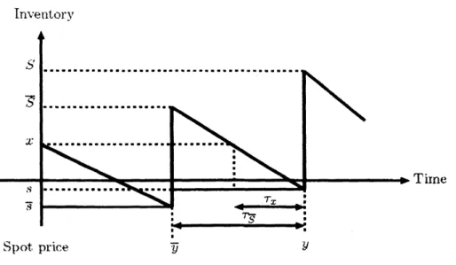
present the model

(2)

Inventorv

Figure 1: Inventory flow

Quasi-variational inequality, and we show in section 4 that there exists anoptimal procure-ment policy which is the type of

an

$(s, S)$ policy. In section 5

we

discuss the

case

of the

specific typc of spot price, and clarifies the impact of the spot price

on

the value function.

Section 6 concludes the paper.

2. Notations and Assumptions

The analysis is ba.sed

on

the following assiimptions:

(i) Time is continuous and inventory is continuously reviewed.

(ii) Demand is $g$ units per umit time in one cycle. Unsatisfied demand is backlogged.

(iii) A critical-level $(s, S, y)$ policy is in place, which

means

that the inventory level $x$ is

drops to an reorder point $s$, then the inventory level increa.ses up to $S$. And then the

next $s$ and $S$

are

determined, ba.sed on the observation of the spot price $y(t)$ at time

$t$

.

Since $s$ and $S$

are

changing at the beginning of each cycle,

we

suppose that

$\overline{s}$ and

3

are

reorder point and order-up-to level for the last cycle, respectively. Therefore, $\overline{S}$

represents the initial inventory level at the beginningof the next cycle, (seeFigiire 1). (iv) The set up cost is $K$ and the unit cost is equal to the spot price $y(\cdot)$

.

The shortage

cost. $p$ and holding cost $q$

are

given by the function $f$:

$f(x)=\{\begin{array}{ll}-px for x<0,qx for x\geq 0.\end{array}$ (1)

(v) The spot price at time $t,$ $y(t)$, follows ageometric Brownian motion, that is,

$dy(t)=y(t)(\mu dt+\sigma dw(t))$

.

(2)

where $w(t)$ follows

a

standard Brownian motion.

A procurement policy consists of a sequence $V=\{(\theta_{i}, \xi_{i}), i=1,2, \cdots\}$of i-th ordering

time $\theta_{i}$ and order quantity $\xi_{i}$. Let $u(x, y)$ be the optimal total expected discounted cost

(3)

price by $y$

.

Then

can

be written

as

$?x(x, y)$ $=$ $\inf_{v^{r}}(E_{y}[\int_{0}^{\infty}f(x(t))e^{-\alpha t}dt+\sum_{i\geq 1}(K+y(\theta_{i})\xi_{i})e^{-\alpha\theta_{i}}]|x(0)=x,$ _$y(0)=y)$

(3)

where the inventory level $x(t)$ is given by

$dx(t)=-gdt+ \sum_{i\geq 1}\xi_{i}\delta(t-\theta_{i})$

.

(4)

with $x(O)=x$ and $\alpha>0$ is interest rate. In _equation _(4), $\delta(\cdot)$ denotes the Dirac fimction,

that is,

$\delta(,\tilde{6})=\{\begin{array}{l}1for z=0,0 otherwise.\end{array}$ (5)

Note that $u(x, y)$ is continuous and everywhere _{differentiable} _in $x$, and also it is twice

differentiable in $y$

.

Our

objective is to find the optimal procurement policy $(s, S)$ _at which the _minimum

value

function

$u$be attained.

3. QVI Problem and Optimal Procurement Policy

In this section,

we

deal with equation (3) as a Quasi-Variational Inequality (QVI) problem (Bensoussan and Lions [4]).

First, if the procurement is not made at least during asmall time interval $(t, t+\epsilon)$, then

we

have following inequation;

$u(x, y)$ $\leq$ $\int^{t+\epsilon}f(x(s))e^{-\alpha(s-t)}ds+u(x(t+\epsilon), y(t+\epsilon,))e^{-\alpha\epsilon}$ . (6)

We can expand the right haiid side of equation (6) up to first order in $\epsilon$ and then we have

$\epsilon f(x)+u(x, y)-g\epsilon.\frac{\partial\uparrow x}{\partial x}+\mu y\epsilon\frac{\partial\tau\iota}{\partial\not\in/}+\frac{1}{2}\epsilon\sigma^{2}y^{2}\frac{\partial^{2_{\uparrow l}}}{\partial\uparrow J^{2}}-\alpha\epsilon u(x, y)+o(\epsilon^{2})$

.

(7)

Hence, making $\epsilon$ tend to $0$, equation (6)

can

be deduced to

$\frac{1}{2}\sigma^{2}y^{2}\frac{\partial^{2_{ll}}}{\partial\not\in J^{2}}+\mu y\frac{\partial_{t}\iota}{\partial\not\in/}-g\frac{\partial?x}{\partial x}-\alpha u\geq-f(x)$

.

(8)

On the other hand, ifthe procurement is made at time $t$, the inventory leveljumps from

$x$ to an $x+\xi$

.

We

assume

that theorder quantity is delivered immediately,

so

the spot price

before the procurement is equal to the price after procurement. Thus,

we

obtain

$u(x, y) \leq K+\inf_{\xi\geq 0}(y(t)\xi+u(x+\xi, y(t)))$

.

(9)

Therefore, the equation (3) is given by a solution of the QVI problem:

niin$(Au+f, \Lambda lu-u)=0$ (10)

where

$Au$$(x, y):= \frac{1}{2}\sigma^{2}y^{2}\frac{\partial^{2}\uparrow\iota}{\partial\uparrow/^{2}}+\mu y\frac{\partial\tau\iota}{\partial\uparrow/}-g\frac{\partial\tau\iota}{\partial x}-au$, (11)

(4)

4. Solution of QVI Problem

In this section, we solve the QVI problem (10) quoted by Sulem [10] in part. We divide the inventory space into two regions; for no procurei$\iota ient$,

$G=\{x\in \mathcal{R}:u(x, y)<Mu(x, y)\}=\{x\in \mathcal{R}:x>s\}$ ₍₁₃₎

then,

we

have

$Au=f$. (14)

And its complement is given by

$\overline{G}=\{x\in \mathcal{R}:u(x, y)=M\uparrow x(x, y)\}=\{x\in \mathcal{R}:x\leq 9\}$ (15)

and for $x\in\overline{C_{7}}$,

we

have

$u(x, y)$ $=$ _{$K+ \inf_{\geq\backslash \xi 0}(y(t)\xi+u(x+\xi, y(t)))$} (16)

$=$ $K+y(t)(S-x)+u(S, y(t))$. (17)

Due to the deterministic demand,

we

take the inventory level aks the elapsed time from

the beginning of the cycle. Thus, we describe the spot price $l/x$ depending

on

the inventory

level $x$.

Since $u$ is continuously differentiable in$x$, in inventoryspace$\overline{G}$, we

can

get

theboundary conditions on $u$.

(i) Continuity of the derivative of$\uparrow\iota$ at the boundary point.9:

$1 inl\frac{\partial\uparrow\iota(x,\uparrow/)}{\partial x}x\downarrow s=-y_{8}$. (18)

(ii) The $infim\iota mi$ in equation (16) is attained at $\overline{S}$:

lin$i^{\underline{\partial\uparrow\iota(:r,y)}}=-\overline{\uparrow/}$

, (19)

$x\uparrow\overline{S}$

$\partial x$

where $\overline{?/}$ is the spot price at the beginning of the cycle.

(iii) $\uparrow\iota$ is continuous at $s$:

$\tau\iota(S, y)=u(s, y)-K-y_{s}(S-s)$. (20)

(iv) The growth condition of $\uparrow\iota$:

$x arrow\infty 1in1\frac{\tau x(x,\uparrow/)}{f(x)}<+\infty$. (21)

To obtain the value function $\uparrow\iota$,

we

solve the partial differential equation (14) with the

initial and boundary conditions (18)-(21). First,

we

set

(5)

(25) This results in the equation

$(l- \mu k+\alpha+\frac{1}{2}k(1-k^{l})\sigma^{2})11’+\frac{\partial w}{\partial\tau}$

$+(( \frac{1}{2}-k)\sigma^{2}-\mu)\frac{\partial_{l1\prime}}{\partial_{\tilde{4}}}-\frac{\sigma^{2}}{2}\frac{\partial^{2}u}{\partial_{\tilde{4}}^{2}’}=f(g\tau+s)e^{-(kz+l\tau)}$ (23)

where

we

choose $k$ and $l$ satisfying

$k=- \frac{1}{\sigma^{2}}(\mu-\frac{1}{2}\sigma^{2})$ , $l=- \frac{1}{2\sigma^{2}}(l^{1}\cdot-\frac{1}{2}\sigma^{2})^{2}-\alpha$

.

(24)

Then,

_{we can}

get the non-homogeneous heat equation

$\frac{\partial w}{\partial\tau}-\frac{\sigma^{2}}{2}\frac{\partial^{2_{?1}}}{\partial\approx 2}=f(g\tau+s)\exp\{\frac{1}{\sigma^{2}}(/\iota-\frac{1}{2}\sigma^{2})z+(\frac{1}{2\sigma^{2}}(\mu-\frac{1}{2}\sigma^{2})^{2}+\alpha)\tau\}$

with

$\uparrow 1)(0, \approx)$ $=$ $e$歩$( \mu-\frac{\sigma^{2}}{2})z\{v(\tau_{S}, \approx)+K+e^{z}(S-s)\}\equiv m(z)$, (26)

$\tau_{6}$ $=$ $\frac{S-s}{g}$

.

(27)

The solution to the diffusion equationproblem is given by

$\uparrow 1)(\tau, z)=\tau\iota)1(\tau, \approx)+\tau r.)2(\tau, z)$_, (28)

where $u$)$1(\tau, z)$ and $\uparrow\iota$)$2(\tau, \approx)$ are solutions offollowing problems:

$\frac{\partial_{T1’ 1}}{\partial\tau}=\frac{\sigma^{2}}{2}\frac{\partial^{2}\uparrow 1J_{1}}{\partial_{\tilde{\sim}}^{2}}$,

$w_{1}(0, z)=rn(z)$, (29)

$\frac{\partial?1\prime_{2}}{\partial\tau}=\frac{\sigma^{2}}{2}\frac{\partial^{2_{llJ_{2}}}}{\partial z^{2}}+l)(\tau, z)$,

$?1\prime_{2}(0, \approx)=0$

.

(30)

Here, we set the right hand side of $e$quation (25) as $f|,(\tau, \approx)$. The solutions $w_{1},$ $w_{2}$ of each

problem (29) and (30) are, respectively, given by

$\uparrow 1\dagger_{1}(\tau,$$\langle’\sim)$ _$=$ $\frac{1}{\sqrt{2\pi\sigma^{2}\tau}}\int_{-\infty}^{\infty}?$

疋$\}1(0)\xi)\exp\{-\frac{(z-\xi)^{2}}{2\sigma^{2_{\mathcal{T}}}}\}d\xi$

$=$ $\frac{1}{\sqrt{2\pi}}e^{n_{-}(\eta_{\overline{k}})}\int_{-\infty}^{\infty}tJ$ $( \tau_{S}\rangle T(\mu-\frac{\sigma^{2}}{2})$ $+\lambda\sigma\sqrt{\mathcal{T}}+Z)e^{-\frac{\lambda^{2}}{2}}d\lambda$

$+Ke^{rz-(\eta,\approx)}+(S-s)e^{n+(\eta.z)}$, (31)

aiid

$\uparrow l.|2(\tau, z)$ $=$ $\frac{1}{\sqrt{2\pi\sigma^{2}}}\int_{0}^{\tau}\frac{1}{\sqrt{\tau-\delta}}(\int_{-\infty}^{\infty}f_{1},(\delta, \xi)\exp(-\frac{(z-\xi)^{2}}{2\sigma^{2}(\tau-\delta)})d\xi)d\delta$

(6)

wliere

$n_{\pm}( \tau, z)=\frac{1}{2\sigma^{2}}(\mu\pm\frac{\sigma^{2}}{2})(\tau(\mu\pm\frac{\sigma^{2}}{2})+2z)$ . (33)

Therefore, from equations (22), (28), (31) and (32), $u(x, y)$

can

be _rewritten $a_{\wedge}s$ follows;

$u(x, y)=e^{-\alpha\tau_{x}}[ \frac{1}{\sqrt{2\pi}}\int_{-\infty}^{\infty}u(S, y_{x}e^{\tau_{x}(\mu-\frac{\sigma^{2}}{2})+\lambda\sigma\sqrt{\tau_{x}}})e^{-\frac{\lambda^{2}}{2}}d\lambda$

$+K+(S-s)_{l/x}e^{\mu\tau_{z}}+ \int_{0}^{\tau_{x}}f(g\delta+s’)e^{\alpha\delta}d\delta]$ . (34)

In the la.st term of equation (34), it can be rewritten as

$D(x)$ $\equiv$ $\int_{0}^{r_{x}}f(g\delta+s)e^{\alpha\delta}d\delta$

$=$ $\{\begin{array}{ll}\alpha 4i(s_{a}-4)+4\alpha(x_{a}-A)e^{\alpha\tau_{x}}+\alpha A_{2}(p+q)e^{-\frac{a}{g}s} for x\geq 0,-p\{(x_{\alpha}^{g}-)e^{\alpha r_{x}}-s+A\alpha\} for x<0,\end{array}$ (35)

(38)

and $D(s)=0$

.

Therefore,

we

have

$u(x, y)$ $=$ $e^{-\alpha\tau_{x}}[E[\uparrow 4(S, \uparrow/xe^{\tau_{x}(\mu-\frac{\sigma^{\underline{Q}}}{2})+\sigma\sqrt{\tau_{x}}X})]+K+(S-s)\tau Jxe^{\mu\tau_{x}}+D(x)]$

$=$ $e^{-\alpha\tau_{x}}[u(S, y)+K+(S-s)y_{x}e^{\mu\tau_{x}}+D(x)]$ ₍₃₆₎

where $X$ is a standard normal random variable.

Lemma 1. The optimal cost$f\uparrow mc$tion $u(x, y)$ is given by

$\uparrow\iota(x, y)$ $=$ $\frac{g}{CY}(\frac{q}{g}\overline{S}+\overline{\uparrow/})\overline{s}\uparrow e^{(/\iota-\alpha)\tau_{x}}-(\iota-\frac{/4}{\alpha})\pi^{-\alpha\tau_{x}}$

(37)

where

$L(x)$ $=$ $\{\begin{array}{l}A\alpha\{(x_{\alpha}-4)-(\overline{S}_{\alpha}-p)e^{\alpha(\eta-\tau_{x})}\}-1i\alpha(x_{\alpha}\text{ノ^{}-g})_{\alpha}-A(\overline{S}_{\alpha}-A)e_{\alpha}^{\alpha(r_{\nabla^{-\tau_{x})}-*(p+q)e^{-\frac{\alpha}{g}x}}}\end{array}$ $forx<0forx\geq 0.$’

Note that $L(x)<0$ for all $x$

.

Remark. Note that equation (37)

can

be reduced to the deterministic-demand

ca.se

of

Sulem’s model when we a.ssume $/.\iota=\sigma=0,$ $y=\overline{y},$ $S=\overline{S}$

.

In this case, the optimal cost

$\tilde{|\iota}(x)$ can be reduced to be

$\tilde{u}(x)$ $=$ $\{\frac{(q+\alpha y)g}{\alpha^{2}}e^{\frac{\alpha s}{g}}-\frac{qg}{\alpha^{2}}\}e^{-\frac{ax}{9}}+\frac{r}{\alpha}x+\frac{rg}{\alpha^{2}}(e^{-\frac{\alpha x}{g}}-1)$ (39)

where

$r$ $=$ $\{\begin{array}{ll}-p for x<0,q for x\geq 0.\end{array}$ (40)

(7)

Next weshow theproperties of$?x$and the existenceof optimal policybased on Benkherouf

[3]. Let us denote $H(x, y)=u(x, y)+?/x^{X}$

.

_{Then, equation (14)}

_can

_{be rewritten} _aks

$g \frac{\partial H}{\partial\prime r,}+\alpha H+l^{\iota\uparrow/x}$ _.

(41) Lemma 3. There exists a pair $(s., S)$ such that .9 and $S$ satisfy equations (18)_$-(21)$

.

Theorem 1.

_If

$(\mu-\alpha)y_{x}+p>0$

for

_$x<0$_, _then an _optimal_policy _{$(s, S)$} _is _solution

_of

the Q VI problem,

an

$d$ the value

of

$(s, S)$ is given by the solution

of

$follo\uparrow ving$ simultaneous

equation:

$\frac{g}{c\nu}(\frac{p}{g}S-\uparrow/s)+\frac{q}{\alpha}(S-\frac{g}{\alpha})+\frac{g}{\alpha}(\overline{\uparrow/}+\frac{q}{\alpha})e^{\alpha(7I^{-\tau s})}+K$

$+ \{/s(1-\frac{/x}{\alpha})/8\pi^{-a\tau}s$ ₍₄₂₎

$\frac{g}{\alpha}(\frac{q}{g}\overline{S}+\overline{\uparrow/})e^{\alpha_{\overline{s}}}-\frac{q}{\alpha}(S-\frac{g}{\alpha})-\frac{g}{a}(\overline{?/}+\frac{q}{\alpha})e^{\alpha(7_{\overline{S}}^{\backslash }-rs)}-D(\overline{S})-K$

$- \{\backslash (1-\frac{\mu}{\alpha})(1-e^{-\alpha\tau s’})\}(S-s)=0$ ₍₄₃₎

Lemma 5. The value $(s, S)$ _satOsfying _equafions ₍₄₂₎ _{and (43) is} _a _unique _solution

_of

_the

Q VIproblem (10).

Theorem 2.

_If

$(\mu-\alpha)y_{x}+p\leq 0$

for

$x<0$ , therp is no solution to the _$QVI$_problem _(10).

5. The Type of

a

Specific Spot Price

Since equations (42) and (43) depend on the spot price $y_{s}$ at the end of cycle, we assume

that the price isequaltothe expectationofspot price at the end of cycle in order to estimate

the total cost at the beginning of cycle. Thus, we assign

$/l_{x}j$ (44)

to equation (37). Then, we have

$u(x)= \frac{g}{\alpha}(\frac{q}{g}\overline{S}+\overline{\iota/})e^{\alpha(\pi^{-r_{x})}}-\frac{l^{1}}{\alpha}\overline{?/}e^{\mu p-\alpha\tau_{x}}(S-s)+L(x)$. (45) Lemma 6. $u(x)$ is increasing in$\overline{?/}for$$l^{l} \leq\frac{1+\alpha\pi^{r_{9}}}{\pi(1+\tau\sigma’)}f$ and is decreasing in $\overline{y}$

for

$\mu>\frac{1\alpha}{\pi(1+\tau s)}$

.

Lemma 7. $u(x)$ is increasing in $\mu$.

6. Concluding Remarks and Further Research

In this paper,

we

showed the existence of

an

optimal policy for the inventory model that

permits the mamifactures to procure the products from the spot market. We obtained the optimal cost fUnction as the solution of Quasi-variational inequality, and showed that there exists

an

optimal procurement policywhich is described by the formof

an

$(s, S)$ policy. For

future research

we

may extend theinventory modelwithprocurement fromspot market into the model where demand also follows diffusion process and incorporate the supply contracts

(8)

References

[1! J. A. Bather: A Continuous Time Inventory Model, Journal

_of

Applied Probability, 3 (1966),

538-549.

[2] L.

Benkherouf

and L. Aggoun:

On a

Stocha.stic

Inventory Model with Deterioration

and Stock-dependent Demand Items, Probability in the Engineering and

_{Informational}

Sciences, 16 (2002), 151-165.

[3] L. Benkherouf:

On a

Stocha.stic Inventory Model with a Generalized Holding Costs,

$E\uparrow\iota ropean$ Journal

of

Operational Research, 182 (2007), 730-737.

[4] A. Bensoussan and J. L. Lions: Impulse Control and Quasi-variational Inequalities,

Gauthier Villar.9, Paris, (1984).

[5] A. Bensoussan, R. H. Liu, and S. P. Sethi: Optimality of an $(s, S)$ policy with

com-pound Poisson and diffusion demaixds: a qua.si-variational inequalities approach, SIAM

Journal on Control and $Optimi\approx ati_{07l},,$ $44$ (2005),

1650-1676.

[6] A. Bar-Ilan and A. Sulem: Explicit Solution ofInventory Problems with Delivery Lags,

Mathematics

_of

Opemtions Research, 20 (1995),

709-720.

[7] A. Goel, and G. J.

Gutierrez:

Integrating spot and futures commodity markets in the optinial procurement policy of

an

a.ssembly-to-order manufacturer, $\uparrow norkin,g$ paper,

Management Department, University ofTexas, Austin, (2004).

[8] X. Guo, P. Tomecek and M. Yuen: Optimal Spot Market Inventory Strategies in the Presence of Cost and Price Risk, working paper, University of Califomia, Berkeley,

(2007).

[9] P. V. O’Neil: Beginning partial differential equations, John Wiley and Sons, New York,

(1999).

[10] A. Sulem: A Solvable-one Dimensional Model of a Difftlsion Inventory System,