A two-scale model for concrete carbonation process in a three dimensional domain (Developments of the theory of evolution equations as the applications to the analysis for nonlinear phenomena)

A

$t_{WO-SCa1emo(\int_{reedi\mathring{m}enszona}^{e1forcncrete}\int^{a}3_{oma1R}^{bonation}}P^{roceSS\ln at}$ 日本女子大学・理学部 愛木豊彦(Toyohiko Aiki)

Department of Mathematical and Physical Sciences, Facultyof Science

Japan Women’sUniversity

名城大学・理工学部 村瀬勇介 ($Y_{11}$snke Murase)

Department of Mathematics, Faculty of Science and Technology

Meijo University

長岡工業高等専門学校・一般教育科 佐藤直紀 (Naoki Sato)

Division of General Education

Nagaoka National College ofTechnology

苫小牧工業高等専門学校・総合学科 熊崎耕太 (Kota Kumazaki)

Department of Natural and Physical Sciences

Tomakomai National College ofTechnology

1

Introduction

Concrete carbonation is

one

ofimportant issues in our real life so that it is necessaryto

elucidateits dynamics. On thissubjectMuntean-Bohmalready proposeda freeboundary

model

on

a

one-dimensionalinterval in [19, 21], and

we

studied the simplified model for

their

one

and established large-time behavior of the free boundary in [4, 5, 6, 7].

The main topic of this paper is concerned with the mathematical model for

con-crete carbonation in athree-dimensional domain, which

was

givenby

Maekawa-Chaube-Kishi[17] and Maekawa-Ishida-Kishi[18] from a civil engineering point of view. The model consists ofthe moisture transport equation and the diffusion equation for carbon

dioxide. In this paper

we

deal with only the former equation and the latter

one

was

discussed in [13, 14, 15].

Here, we show

our

first model for moisture transport, briefly, since the detail of the

modeling was mentioned in [1]. We suppose that the concrete occupies the bounded domain $\Omega\subseteq \mathbb{R}$ with the smooth boundary. Let

$\rho_{w}$ be the density of water, $s$ be

the degree of saturation and $h$ be the relative humidity. From observations for real

experimental

_result.

$s$ it is pointed out that the graph of the relationship between $\mathcal{S}$ and

$h$ is close to

one

ofhysteresis with anti-clockwise trend in [17, 18]. Accordingly, from a

phenomenological point of view

we

approximated the relationship with a play operator

in [2, 3, 1, 16]. Then

we

obtain the following system:

$\rho_{w}h,.-div(g(h)\nabla h)=sf$ in $Q(T):=(O,T)\cross\Omega$, (1.1)

$s_{t}+\partial I(h;s)\ni O$ in $Q(T)$, (1.2)

$h=h_{b}$ on $\Gamma(T):=(O,T)\cross\partial\Omega$, (1.3)

where$f$is

a

givenfunction

on

$Q(T)$ and indicates the generationofwater by thechemical

reaction, $h_{b}$ and $h_{0}$ be given function on $Q(T)$ and

$\Omega$

, respectively, and $g$ is acontinuous

function

on

$(0, \infty)$ (see Figure 1) and describes the diffusion coefficient depending

on

the humidity. The ordinary

differential

equation (1.2) is

one

ofcharacterization for the

play operator (see [10, 25] and Figure 2), and $I$ is the indicator function of the closed

interval $[f_{*}(h), f^{*}(h)]$ and $\partial I$ is its subdifferential, where $f_{*}$ and $f^{*}$

are

lower and upper

branches of the hysteresis loop, respectively.

Figure 2: Graph of play operator Figure 1: Diffusion coefficient

For the system $(.1.1)\sim(1.4)$ $(:=CP)$

we

already proved:

Theorem 1.1. ([2,3,16])

(Al) $g\in C^{2}((0, \infty g(r)\geq g_{0}$

for

$r>0$, where$g_{0}$ is apositive constant.

$(A2)f\in L^{\infty}(Q(T))$

,

$f_{t}\in L^{2}(0, T_{1}L^{2}(\Omega))$ and $f\geq 0a.e$

.

on

$Q(T)$.

$(A3)f_{*},$$f^{*}\in C^{2}(\mathbb{R})\cap W^{2,\infty}(\mathbb{R})$, $0\leq f_{*}\leq f^{*}\leq s_{*}$, where $s_{*}$ is

a

positive constant.

$(A4)h_{b}\in C^{2,1}(\overline{Q(T)})$, $h_{bt}\in L^{2}(0, T;H^{2}(\Omega))$, $h_{b}\geq\delta_{0}>0a.e$.

on

$\Gamma(T)$, $h_{0}\in$ $H^{2}(\Omega)\cap W^{1,\infty}(\Omega)$, $\mathcal{S}_{0}\in H^{1}(\Omega)\cap L^{\infty}(\Omega)$, $h_{0}\geq\delta_{0}a.e.$ $on\Omega,$ _{$h_{b}(0)=h_{0}a.e.$} $on\partial\Omega,$

$f_{*}(h_{0})\leq s_{0}\leq f^{*}(h_{0})a.e$. on $\Omega$

, where $\delta_{0}$ is a positive constant.

If

$(Al)\sim(A4)$ hold, then $CP$ has a unique solution on $[O, T].$

As

a

next step of this research we will consider the following equation

as

a

mathe-matical description for moisture transport:

$p_{w}h_{t}-div((g(h)+\phi(1-s))\nabla h)=sf$, (1.5)

where $\phi$ is the porosity function given on $Q(T)$. Since it is not easy to obtain

some

uniform estimates for $\nabla s$ from (1.2) in order to solve theinitial boundaryvalue problem

for (1.5), we propose

a

new two-scale model for moisture transport. The exact form

will be given in the next section. Here,

we

note that the model consists of two system defined on the

macro

and micro domains. Particularly, thesystem on the micro domain is a one-dimensional free boundary problem.

The two-scale model with partial differential equations was alreadystudied by many

withhomogenization (see [20,24,11,12,8 We remark that both

a

macro

and amicro

systems

are

considered

on a

fixeddomain in allof theseresults, namely, the homogeneous domain $is$ assumed. In

our

model

we can deal

with non-homogeneous

case.

Thepurposes ofthispaper

are

tointroduce the idea of two-scalemodelingformoisture

transport in Section 2 $a\alpha ld$ to _{$establish_{\sim}the$} existence, uniqueness and the large time

behavior of a solution of the free boundary problem in Section 3. Also, thesummary is shown in the samesection.

2

Two-scale

model

In this section we show our two-scale model for moisture transport. Let $\zeta$) $\subseteq \mathbb{R}^{3}$ be

a

bounded (macro) domain occupied with concrete, and $t$ be the time,

$0<t<T.$

We suppose that for any $\xi\in\Omega$ one pore is corresponded and regard the pore

as

the

interval (micro domain) $(0,1)$ decomposed to the water region $(O, s(t, \xi))$ and the air

region $(s(t, \xi), 1)$ (see Figure $3\rangle$. Since the physical definition of the degreeofsaturation

$s$ is the ratio of water

area

to the total volume of each pore in the porous media, the

degree of saturation is given by $s$ in our formulation,

Figure 3:

Let $u(t, \xi, x)$ be the relative humidity at the place $x$ in the air region. We impose

a diffusion equation for $u$ and the Dirichlet boundary condition at the fixed boundary

$x=1$. This boundarycondition

means

thatthe airofeach microdomainconnects to the

air of the

macro

domain at $x=1$. The free boundary condition

was

already discussed

in [22, 23, 9] so that

we

omit its physical interpretation. Then

we can

get the following

free boundary problem for each $\xi\in\Omega$ and

a

function $h$

on

_$Q(T)$: The problem $FBP(h)$

Figure 4) sat\’isfying

$\rho_{a}u_{t}-\kappa u_{xx}=0$

on

$(s(t,\xi), 1)$ for $0<t<T$, (2.1)

$u(t,\xi, 1)=h(t,\xi)$ for $0<t<T$, (2.2) $\kappa u_{x}(t,\xi, s(t))=(\rho_{w}-\rho_{a}u(t,\xi, s(t, \xi)))s’(t, \xi)$ for

$0<t<T$

, (2.3) $s’(t, \xi)=a(u(t_{\mathcal{S}}(t_{\mathfrak{j}}\xi))-\varphi(\mathcal{S}(t,\xi for 0<t<T,$ (2.4)

$\mathcal{S}(0,\xi)=s_{0}(\xi)$,$u(O, \xi, x)=u_{0}(\xi, x)$ for $s_{0}(\xi)\leq x\leq 1$, (2.5)

where $\rho_{a}$ is the density of water in air,

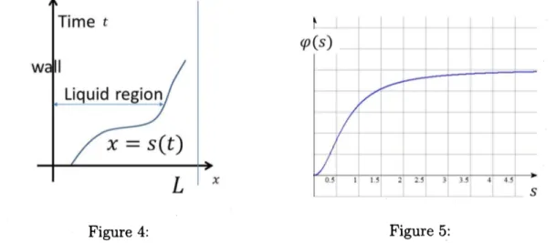
$\kappa$ is a diffusion constant, the positive constant $a$ indicates the growth rate of water region, $\varphi$ :

$\mathbb{R}arrow \mathbb{R}$ is bounded and continuous, and

$\mathcal{S}_{0}$ and $u_{0}$

are

initial data of $s$ and $u$, respectively. Here,

we

give Figure 5

as

a graph of

the typical example of $\varphi$

.

Also, for each $\xi$

we

denote by $S$ the mapping from

$h$ $\xi$) to the free boundary $s$ $\xi$), namely, $S(h(\cdot, \xi))=s$

means

that $s$is the free boundary of the

problem$FBP(h(\cdot,\xi$

$\}$

Figure 4: Figure 5:

Thus

we

obtain the two-scale model MP for moisture transport as follows: This

problem is to find

a

triple of functions $h$ and $s$

on

$Q(T)$ and a function $u$

on

$\Sigma_{s}(T)$ $:=$ $\{(t, \xi, x) : 0<t<T, \xi\in\Omega, s(l)<x<1\}$ satisfying

$\rho_{w}h_{t}-div(g(h)\nabla h)=sf$ in $Q(T)$, (2.6)

$h=h_{b} on\Gamma(T) , h(O)=h_{0} on\Omega$, (2.7)

$\rho_{a}u_{t}-\kappa u_{xx}=0$ on $(s(t, \xi), 1)$ for $0<t<T$, (2.8)

$u(t,\xi, 1)=h(t, \xi)$ for $(t,\xi)\in Q(T)$, (2.9) $(\rho_{w}-\rho_{a}u(t, \xi, s(t,\xi)))s’(t, \xi)=\kappa u_{x}(t, \xi, s(l))$ for

$0<t<T$

, (2.10) $s’(t, \xi)=a(u(t, \xi, s(t, \xi))-\varphi(s(t, \xi for (t, \xi)\in Q(T)$, (2.11)

$s(O,\xi)=s_{0}(\xi)$,$u(O, \xi, x)=u_{0}(\xi, x)$ for $s_{0}\leq x\leq 1,$$\xi\in\Omega$

.

(2.12)

3

Results

on

the free

boundary

problem

and

sum-mary

In this section

we

show

our

recent results on FBP. For simplicity

we

omit the

macro

parameter $\xi$. First,

we

give assumptions for $\varphi,$ $a_{7}\rho_{w},$ $\rho_{a}$ and etc.

(H1) $\varphi\in C^{1}(\mathbb{R})\cap W^{1,\infty}(\mathbb{R})$, $\varphi=0$

on

$(-\infty, 0], \varphi\leq 1 on \mathbb{R}, \varphi’(r)>0$

on

$(0,1]$, and

$a$ is

a

positive constant.

(H2) $p_{w}$ and $\rho_{a}$

are

positive

constants

with

$p_{w}>2p_{a)}\rho_{w}\geq p_{a}(|\varphi’|_{L^{\infty}(\mathbb{R})}+2)$ and $9ap_{a}^{2}\leq\kappa\rho_{w},$

(H3) $h\in W_{loc}^{1,2}([0, \infty h’\in L^{1}(0,\infty\rangle\cap L^{2}(0, \infty),$ $\}im_{tarrow\infty}h(t)=h_{\infty},$ $h-h_{\infty}\in$

$L^{1}(0, \infty)$, $0\leq h\leq h_{*}<\varphi(1)$ on $(0, \infty)$, where $h_{*}$ is

a

positive constant.

(H4) $0\leq s_{0}<1,$ $u_{0}\in W^{1,2}(s_{\zeta)}, 1)$, _{$u_{0}(1)=h(0)$}, $0\leq u_{1\}}\leq 1$ on $[s_{(\}}$, 1$].$

Then we have proved:

Theorem 3.1. $([22, 9J)$

_If

$(H1)\sim(H4)$ hold, then the problem $FBP(h)$ _has

a

solution

$\{s, u\}$

on

[$0,$$\infty\rangle$ and there exists a constant $s^{*}\in(0,1)$ such that $0\leq s\leq s^{*}$

on

$[0, \infty$). Moreover, $\mathcal{S}(i)arrow s_{\infty}$ and $u(t, (1-y)s(t)+y)arrow h_{\infty}$

for

$y\in[O$,1$]$

as

$tarrow\infty$, where

$s_{\infty}\in[O$, 1$)$ with $\varphi(s_{\infty})=h_{\infty},$

At the end of this paper, we list future works on the two-scale model for concrete

carbonation.

$\bullet$ As mentioned in Theorem 3.1, FBP has

a

global solution in time. Then, since

we

have a chance to solve MP, we aretrying it,

now.

$\bullet$ After

we

solve MP,

we

will consider

a

system consisting of (1.5) and $S(h)=s.$

Furthermore, we would like to deal with a couple of the system and the diffusion

equation for carbon dioxide.

$\bullet$ Recently,

we can

showthe existence of

a

periodic solution of FBP. But, the

unique-nessof the periodic solution isstill open. Now, weguess that it is effective todefine asolution in aweaksense for its proof. However, the definition of

a

weak solution of FBP is not established, yet.

$\bullet$ We have

some

conjectures

on

the convergence rate of

a

solution of FBP from the

observationsto

our

numerical resultsin [9]

so

that we wouldliketo guarantee those

conjectures.

References

[1] T. Aiki, K. Kumazaki, Mathematical modeling of concrete carbonation process with hysyteresis effect. Surikaisekikenkyifsho Kokyuroku, No. 1792(2012), 98-107.

[2] T. Aiki, K. Kumazaki, Mathematical model for hysteresisphenomenon in moisture

[3] T. Aiki, K. Kumazaki, Well-posedness

of

a mathematical model for moisture

trans-port appearing in concrete carbonation process, Adv. Math.

Sci.

Appl., 21(2011),

361-381.

[4] T. Aiki,A. Muntean, Existence anduniquenessofsolutionsto

a

mathematicalmodel

predicting service life of concrete structures, Adv. Math. Sci. Appl., 19(2009),

109-129.

[5] T. Aiki, A. Muntean, Large time behavior of solutions to concrete carbonation

problem, Communications

on

Pure and Applied Analysis, Vol. 9, $(2010)1117-1129.$

[6] T. Aiki, A. Muntean, A free-boundary problem for concrete carbonation: Rigorous

justification of $\sqrt{t}$

-law of propagation, Interfaces and

Free

Bound., 15(2012),

167-180.

[7] T. Aiki, A. Muntean, Large-time asymptotics of moving-reaction interfaces involv-ing nonlinear Henry’s law and time-dependent Dirichlet $data_{\}}$ Nonlinear Anal.,

93(2013),

3-14.

[8] T. Aiki, A. Muntean, Large-time behavior of

a

two-scale semilinear

reaction-diffusion system for concretesulfatation, Math. MethodsAppl. Sci., 38(2015),

1451-1464.

[9] T. Aiki, Y. Murase, On a large time behavior of a solution to a one-dimensional free boundary problem for adsorption phenomena, in preparation.

[10] M.

Brokate

andJ. Sprekels, Hysteresis and Phase $7\succ$ansitions, Springer, Appl. Math.

Sci.$\rangle 121$, 1996.

[11] V. Chalupeck\’y, T. Fatima, and A. Muntean. Numerical study of

a

fast

micro-macro

mass

transfer limit: The

case

ofsulfate attack in

sewer

pipes. J.

_of

Math-for-Industry, $2B:171-181$, 2010.

[12] T. Fatima, A.

Muntean

and T. Aiki. Distributed space scales in a semilinear

reaction-diffusion system including

a

parabolic variational inequality: A

well-posedness study, Adv. Math. Sci. Appl. 22(2012), 295-318.

[13] K. Kumazaki, A mathematical model of carbon dioxide transport in concrete

car-bonation process. Discrete Contin. Dyn. Syst. Ser. $S7$ _(2014), no. 1, 113–125.

[14] K. Kumazaki, Large time behavior of a solution of carbon dioxide transport model

in concrete carbonation process. J. Differential Equations, 257(2014), 2136-2158.

[15] K. Kumazaki, Exponential decayofasolution forsomeparabolicequation involving

a time nonlocal term, Math. Bohem., 140(2015), 129-137.

[16] K. Kumazaki, T. Aiki, Uniqueness of a solution for some parabolic type equation

with hysteresis in three dimensions. Networks and Heterogeneous Media, 9(2014),

[17] K. Maekawa, R. Chaube, T. Kishi, Modeling

_of

concrete performance, Taylor and

Francis, 1999.

[18] K. Maekawa, $\ulcorner r$

. Ishida, $\prime r$

. Kishi, Multi-scale modeling of concrete performance,

Journal ofAdvanced Concrete Technology, 1(2003),

91-126.

[19] A. Muntean, A moving-boundary problem: Modeling, analysis and simulation of

concrete carbonation, Cuvillier Verlag, G\"otingen, 2006. $PhD$ thesis, Faculty of

Mathematics, University ofBremen, Germany.

[20] A. Muntean and M. Neuss-Radu,

A multiscale

Galerkin approach for

a

class of

non-linear coupled

reaction-diffusion

systems in complex media, J. Math. Anal. Appl.,

371(2010),

705-718.

[21] A. Muntean, M. B\"ohm, A moving-boundary problem for concrete carbonation:

globalexistence anduniqueness ofsolutions,

Journal

of Mathematical Analysis and

Applications, $350\langle 1$)$(2009)$, 234-251.

[22] N. Sato, T. Aiki, Y. Murase, K. Shirakawa, A

mathematical

model for

a

hys-teresis appearing in adsorption phenomena, Surikaisekikenkyusho Kokyuroku, No. 1856(2013), $1arrow 11.$

[23] N. Sato, T. Aiki, Y. Murase, K. Shirakawa, A

one

dimensional

freeboundary

prob-lem for adsorption phenomena, Netw. Heterog. Media, 9(2014),

655-668.

$|24]$ T. Fatima and N. Arab and E. P. Zemskov and A. Muntean, Homogenization of a

reaction-diffusion system modeling sulfate corrosion in locally-periodic perforated

domains, J. Eng. Math., $69(2011)$,

261-276.

[25] A. Visintin,

_{Differential}

Modczls

_of

Hysteresis, Appl. Math. Sci., Vol. 111, Springer-Verlag, Berlin, 1993.