Bifurcation structure of the stationary solution set to a strongly coupled diffusion system(Mathematical Models of Phenomena and Evolution Equations)

Bifurcation

structure

of

the

stationary

solution

set

to

a

strongly

coupled

diffusion system

Kousuke

KUTO

(久藤

衡介

) *

Department of Intelligent

Mechanical Engineering

Faculty of

Engineering,

Fukuoka

Institute

of

Technology

(

福岡工業大学工学部知能機械工学科

)

Abstract

Westudy thepositive stationary solutionset ofastrongly coupled diffusion system

with the Lotka-Volterra reaction term. We obtain the bifurcation branch of the

positivesolutions,whichextends globally with respecttoabifurcation parameter.

Furthermore, by the analysis for the shadow systems,

we

derive the nonlinear

diffisioneffectof

on

thepositivesolution branch.

1 Introduction

Many

reaction-diffision

modelshave beenproposedtodescribethepopulation

dy-namics in

various

ecological situations. Inparticular, the

nonlinear-diffision

systems

withffieLotka-Volterra

interaction

terms have beenextensively studiedbymany

math-enaticians, sincetheadvocated

wgrk

by$\mathrm{S}\mathrm{b}_{\wedge}\mathrm{i}\mathrm{g}\mathrm{e}\mathrm{s}\mathrm{a}\mathrm{d}\mathrm{a}- \mathrm{K}\mathrm{a}\mathrm{w}\mathrm{a}\mathrm{s}\mathrm{a}\mathrm{k}\mathrm{i}- \mathrm{T}\mathrm{e}\mathrm{r}\mathrm{a}\mathrm{m}\mathrm{o}\mathrm{t}\mathrm{o}[19]$

.

Inffiisarticle,

we

focus

on

ffie following stronglycoupled diffisionsystemwiththe

prey-predator interactionterms:

(P)$\{$

$u_{t}=\Delta u+u(a-u-cv)$ in $\Omega \mathrm{x}(0, \infty)$,

$v_{t}= \Delta[(\mu+\frac{1}{1+\beta u})\not\in+v(b+du-v)$ in $\Omega \mathrm{x}$ $(0, \infty)$,

$u=v$ $=0$

on

$\partial\Omega \mathrm{x}$ $(0, \infty)$, $u(\cdot,t)=u_{0}\geq 0$, $v(\cdot, t)=v_{0}\geq 0$

on

$\Omega$,

where

0

is

a

bounded domain in $R^{N}$ with

a

smooth boundary

an

; a,b,c,d, and$\mu$

are

all positiveconstants; $\beta$ is

a

nonnegative constant. System (P) is

a

prey-predator

model, _{From the ecologicalpointof}view,the unknownfunctions $u$and$v$,respectively,

denotethe population densitiesof

prey

andpredatorspecies which

are

interacting and

migrating inthe

same

habitat$\Omega$. Inthereactionterms,_$a$and$b$representthebirthrates

ofthe respective species, $c$ and $d$ denote the prey-predator interactions. In the

sec-ond equation, thestronglycoupled diffusion term$\Delta(\frac{v}{1+\beta u})$ models

a

situation in which

thepopulation

pressure

of predatorspecies weakensin the high density place of

prey

species. On the solvability of(P), Le.Dung [8] has recently found theglobal attractor

for

a

class of thequasilinear parabolic systems involving(P).So itbecomes

more

inter-estingto study the dynamicalstructureforthe solutionsetof(P). As the beginningof

the study,

we

have beenanalyzing for the stationarysolution setof(P), since [10]. To

myknowledge, there

are

few works

on

this fractional type of densitydependence

dif-fusions inthe field ofreaction-diffusionsystems. Itshouldbenoted that

our

nonlinear

diffusiontermisdifferentfrom theusualcross-diffusiontermproposed by [19].

Our

purpose

istoderive the global bifurcation structure of the stationary solution

set. Then

we

will discuss the associatestationaryproblemwith(P);

(SP)$\{$

$\Delta u+u(a-u-cv)$ $=0$ in $\Omega$,

$\Delta||(\mu+\frac{1}{1+\beta u})\not\in+v(b+du-v)=0$ in $\Omega$,

$u=v$ $=0$

on

an.

Among otherthings,

we are

interested in thepositive solutions of(SP). Itis said that

$(u, v)$ is

a

positive solution ifboth $u>0$ and $v$ $>0$ satisfy (SP). From the viewpoint

of theprey-predatormodel,

a

positivesolution$(u, v)$implies

a

coexistencesteady state.

Hence,itis

an

importantproblemtoderivethepositivesolution setof(SP).

Inordertostudythepositivesolutionset,

_we

need

some

notations. Henceforth,

we

will

use &i

(q)todenotethe leasteigenvalueof theproblem

$-\Delta u+q(x)u=\lambda u$ in $\Omega$,

u

$=0$

on

an,

where$q(x)$ is

a

continuous function in$\overline{\Omega}$

.

We simply vite $\lambda_{1}$ instead of$\lambda_{1}(0)$

.

It is

well knownthat thefollowingproblem

$\Delta u+u(a-u)=0$ in $\Omega$, u$=0$

on

an

(1.1)

has

a

unique positive solution$u=\theta_{a}$ifandonly if$a>\lambda_{1}$

.

Hence,(SP)has

a

semitrivial

solution$(u,v)$ $=(9\mathrm{a},0)$ if$a$ $>\lambda_{1}$

.

Furthermoreitis easily verified that(SP)has another

semitrivial solution$(u, v)=(0,0/+1)\theta_{b/\psi+1)})$if$b>(\mu+1)\mathrm{A}\mathrm{i}$, Here,$\theta_{b/\{\mu+1\}}$represents

a

positivesolution of(1.1)with$a$replaced by$b/(\mu+1)$

.

Theusual

norms

of the

spaces

$L^{p}(\Omega)$for_{$p\in[1, \infty)$} and$C(\overline{\Omega})$

are

definedby

$|[u||_{p}:=( \int_{\Omega}|u(x)|^{p}dx)^{1/p}$ and

2

Positive

Solution

Set

2.1

Coexistence

Region

Inthisarticle,

we are

restricted

on

the

case

b$>(\mu+1)\lambda_{1}$

.

The first theoremgives

a

sufficient

con

ditionof the existence ofpositivesolutions:

Theorem

2.1

([10]), Let$a^{*}=\lambda_{1}(c\omega+1)\theta_{b/\{\mu+1)})$

.

$Ifb>(\mu+1)\lambda_{1}$, (SP)has

a

positive

so-lution

_for

$a>a^{*}$

.

From the

bifurcation

structurepoint

of

view, thepositive solutionset

of

(SP)contains

a

local

_bifurcation

branch$\Gamma=\{(u(s),v(s),a(s))\in X\mathrm{x} R : s\in(0,\delta)\}$,

such that $(u(0), v(0),a(0))=(0,(\mathrm{p}+1)\theta_{b/\{\mu+1\rangle},a^{*})$. Furthermore, $\Gamma$

can

be extended

globally withrespectto$a(arrow\infty)$

as a

positive solution branch

of

(SP).

Weremarkthattheabove bifurcationpoint

$a^{*}=\lambda_{1}(c\phi+1)\theta_{b/(u+1)})$ (2.1)

depends

on

$(b, c,\mu)$,butisindependent$\mathrm{o}\mathrm{f}\beta$

.

Furthermore in [10,Lemma2.3],

we

have

proved thatfor any fixed $(\mathrm{c},/\mathrm{i})$, $a^{*}=a^{l}(b)$ is

a

monotone increasing smoothfunction

with respect to $b>(\mu+1)\lambda_{1}$ such that $\lim_{b\backslash \zeta\mu+1)\lambda_{1}}a^{*}(b)=\lambda_{1}$ and $\lim_{b\prec\infty}a^{*}(b)=$

$\infty$

.

Theorem

2.1

enables

us

to find the coexistence region

on

the $(a,b)$

space.

By

the monotone property of the

curve

$a=a^{*}(b)$ (Theorem 2.1),

one can

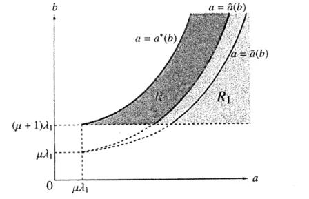
deducethat if

$(a,b)$ lies in the region surrounded by $a=a^{*}(b)$ and $b=(\mu+1)\lambda_{1}$, then (SP) has

a positive

solution (see the region $R_{1}\cup R_{2}$ in Figure1). This region ,$\mathrm{i}\mathrm{n}$

case

$\beta=0$,

corresponds tothe exact coexistence region shown by L\’opez-G6mez andPardo [15].

Fromtheviewpointofthebifurcationtheory,positive solutions bifurcatefrom$(u, v)$ $=$

$(0, y +1)\theta_{b/(\mu+1)})$when $(a, b)$

moves

across

$a=a^{*}(b)$.

2.2

Asymptotic Behavior

of

Positive Solutions

as

$\beta\sim$ $\infty$

Next, Iwill derive the nonlinear effectof large$\beta$

on

the

positive

solution set. For

thesake of thederivation,

we

will introduce two shadowsystems

as

$73arrow$ oo in (SP).

We

assume

that$\psi_{n}$

}

isany positive

sequence

with$\lim_{n\prec\infty}\beta_{n}=\infty$,andthat

$\{(u_{n},v_{n})\}$ isany

positive

solution

sequence

of (SP) with$\beta=\beta_{n}$

.

With

some

suitable assumptions,

we

will

prove

that

one

ofthe following twosituations necessarily

occurs:

(i) There exists

a

certain positive

solution $(u,v)$of

$\{$

$\Delta u+u(a-u-cv)=0$ in $\Omega$,

$\mu\Delta v+v(b+du-v)=0$ in $\Omega$,

$u=v$$=0$

on

an,

(2.2)

such that$\lim_{narrow\infty}(u_{n},v_{n})=(u,$v) in

(ii) Thereexists

a

certain positivesolution$(w, \mathrm{v})$ of

$\{$

$\Delta w$$+w(a-cv)$ $=0$ in $\Omega$,

$\Delta[(\mu+\frac{1}{1+w})v]+v(b-v)=0$ in 0, $w$$=v$ $=0$

on

$\partial\Omega$,

(2.3)

suchthat$\lim_{narrow\infty}(\beta_{nn’ n}u\iota\})=(w,$v) in

$C(\overline{\Omega})^{2}$,passingto

a

subsequence.

Our

convergence

result (Theorem 4.1) will also

ensure

that if$\beta$ is sufhciently large,

any

positive solution of (SP)

can

be approximated by

a

suitable positive solution of

either (2.2)

or

(23). Hence itisnatural to ask which of(2.2) and(23) (orboth)

can

characterizepositive solutions of(SP),accordingtoeachcoefficientvalue.

Thepositivesolution setofthe firstshadowsystem(2.2)has beenextensively

stud-ied by

many

mathematicians (e.g., [2], [4], [5], [6], [13], [14], [15], [16], [20]). As

a

summary

oftheir all results,

we

_know the next result

on

the positive solution set of

(2.2):

Theorem 2.2, _Let

a

$=\lambda_{1}(c\mu\theta_{b/\mu})$

.

Then (2.2) has

a

positive solution

if

and only

if

a>\^a. From the

_bifurcation

structurepoint

_of

view, the positive solution set

_of

(2.2)

contains

a

local

_bifurcation

branch$\Gamma_{1}=\{(\mathrm{w}(\mathrm{s}),\mathrm{v}(\mathrm{s}),\mathrm{a}(\mathrm{s}))\in X\mathrm{x} R : s\in(0,\delta)\}$, such

that$(u(0),v(0),a(0))=(0,\mu\theta_{b/\rho},\text{\^{a}})$. Furthermore, $\Gamma_{1}$

can

be extendedin the direction

a>\^a

_{as an}

_{unboundedpositive solution branch}

_of

(22).

Here

we

note that for any fixed $(\mathrm{c},/\mathrm{i})$, $\text{\^{a}}=\lambda_{1}(c\mu\theta_{b/\mu})$ is

a

monotone increasing

smoothfunctionwithrespectto$b>\mu\lambda_{1}$,suchthat$\lim_{b\forall\lambda_{\mathrm{t}}}\mathrm{a}(\mathrm{b})=\lambda_{1}$and$\lim_{barrow\infty}$

\^a(b)=

$\infty$

.

Furthermore,it

can

beverified that_{$a^{*}(b)<\ (\mathrm{b})$}for all_{$b>(\mu+1)\lambda_{1}$} (seeFigure 1).

Hence, it becomes

a

crucialpart ofthis article to studythepositivesolution setof

the second shadow system (23). By regarding $a$

as a

bifurcation parameter,

we

will

show thatthebranch ofthepositivesolutionsetof(2.3)bifurcatesfrom the semitrivial

solution with $lB$ $\equiv 0$ at_$a=a^{*}$, and

moreover

that this branch extends globally and

blows

up

with respectto $||w||_{\infty}$ ata=\^a:

Theorem2,3 ([12]). Suppose that$b>(\mu+1)\lambda_{1}$. Positive solutions

of

(2.3)

bifurcate

from

thesemitrivialsolution

curve

$\{(0, \mathrm{Q}l +1)\theta_{b/(u+1)},a) : a\in R_{+}\}$

if

and only

if

$a=a^{*}$

.

To beprecise, allpositive solutions

_of

(52)

near

(0,(ju $+1$₎ $\theta_{b/\zeta\mu+1)}$,$a^{*}$) $\in X\mathrm{x}$ $R_{+}$

can

beparameterized

as

$\Gamma_{2}=\{(w(s),v(s),a(s))\in X\mathrm{x} R_{+} : s\in(0,\delta)\}$, such that

$(w(0),v(0),a(0))=(0,\mu\theta_{b/\mu}, \text{\^{a}})$

.

Furthermore, $\Gamma_{2}(\subset X\mathrm{x} R_{+})$

can

be extended

as an

unboundedpositive solution branch (of (23)), which

contains an

unbounded smooth

curve

which isparameterized by $a$; $(\mathrm{w}(\mathrm{a}), \mathrm{v}(\mathrm{a})$ $)\in X\mathrm{x}$ [\^a-\kappa ,

\^a)}

with

a

cenain

positive number$\kappa$

.

Here, $(w(a), v(a))$is

a

smooth

function

such that

$\lim_{a\nearrow\hat{a}}||w(a)|\}_{\infty}=\infty,\lim_{a\nearrow\hat{a}}v(a\grave{)}=\mu\theta_{b/\mu}$ in

Furthermore, it

can

be proved that (2.3) has

no

positive solution if $a\geq$

a

$:=$

$\lambda_{1}(c\mu^{-1}(\mu+1)^{\gamma}\sim\theta_{b/\mu})$. Here,

we

note that$\tilde{a}=\lambda_{1}(c\mu.(\mathrm{J}p +1)^{9}\sim\theta_{b/\mu})$ is also

a

monotone

increasingsmooth function for$b>\mu\lambda_{1}$,such that$\lim_{b\backslash _{\mu\lambda_{\mathrm{I}}}}$ $\text{\^{a}}\langle b$) $=\lambda_{\mathrm{t}}$ and$\lim_{barrow\infty}$\^a(b)=

$\infty$. Furthermore, itholds that$a^{*}(b)<\mathrm{a}(\mathrm{b})<\tilde{a}(b)$forall$b>(\mu+1)\lambda_{1}$ (seeFigure 1).

Consequently, it follows thatif$a\in(a^{*},\text{\^{a}})$, (2.3) has at least

one

positive solution

while (2.2) has

no

positive solution, and that if$a>\overline{a}$, (2.3) has

no

positive solution

while (2.2) has at least

one

positive solution. Ow ing to such studies

on

the shadow

systems,

we

will

prove

theapproximateresultin large$\beta$

case:

Theorem

2.4

([12]). Supposethat $\{(u_{n}, v_{n})\}$ is anypositive solution sequence

of

(SP)

will$\beta=\beta_{n}$ and

,$\lim_{\iotaarrow\infty}\beta_{n}=\infty$

.

Let

$\epsilon$and 6 bearbitrarysmall positive numbers. Then,

thereexistpositive numbers

a

$>a^{4}(>\lambda_{1})$ suchthat

if

$a\in(a^{*}, \text{\^{a}}-\delta 1\cup [\hat{a}+\delta, \infty)$, $b>$

$(p +1)\lambda$

.

and$n$ is sufficiently large, eitherthefollowing situation(i)or(ii)necessarily

occurs

:

(i) There existsa certainpositive solution $(u, v)$

of

(2.2)such that

$\mathrm{m}_{X\in}|u\frac{\mathrm{a}\mathrm{x}}{\Omega},$‘$(x)-u(x)|+\mathrm{m}_{X\epsilon^{\frac{\mathrm{a}\mathrm{x}}{\Omega}}}|v_{n}(x)-v(x)|<\epsilon$.

(ii) There exists

a

certainpositive solution $(w, v)$

of

(2.3)such that

$\mathrm{m}_{\lambda\in}\frac{\mathrm{a}\mathrm{x}}{\Omega}|\beta_{r\iota}u_{\mathit{1}},(x)$$-w(x)|+\mathrm{m}_{X\epsilon^{\frac{\mathrm{a}\mathrm{x}}{\Omega}}}|v_{n}(x)-v(x)|<\epsilon$.

Furthe rnore, there existsanumber$\tilde{a}(>\hat{a})$suchthat

if

$\mathrm{a}\in$ [$\tilde{a}_{\backslash }\infty)$, the situation

of

(ii)

can not occur, and

_if

$a\in(a^{*}$

.a

$-\delta$], thesituation

of

(i) can notoccur.

Figure

1:

Theregion$R_{\mathrm{J}}$ givestheexactcoexistence regionfor(2.2). The region

3

A

Priori

Estimates

In this subsection,

we

introduce

a

semilinear elliptic system equivalent to (SP),

and give

some a

prioriestimates forpositivesolutions of the semilinearsystem([10]).

These

a

priori estimates willplay

an

important role inthesucceeding sections. Since

we are

restricted

on

nonnegative solutions, it is convenientto introduce theunknown

function$V$by

$V=( \mu+\frac{1}{1+\beta u})v$

.

(3.1)

There is

a

one-to-one correspondence between $(u,v)\geq 0$and $(u, V)\geq 0$

.

Then, (SP) is

rewritteninthefollowing equivalent form:

(EP) $\{$

$\Delta u+u(a-u-cv)=0$ in $\Omega$,

$\Delta V+\nu(b+du-v)=0$ in $\Omega$,

$u=V=0$

on

$dn$,

where

v

$=v(u,$V) _{is understood}

as

the function of (u, V) defined by (3.1). Itis easyto

show that(EP)has twosemitrivialsolutions

(u,$V)=(\theta_{a},0)$ for

a

$>\lambda_{1}$ and (u,$V)=(0, \psi +1)^{2}\theta_{b/(u+1)})$ for b_{$>(\mu+1)\lambda_{1}$},

in addition to the trivial solution (u,$V)=(0,$0). _{We obtain} the following

a

priori

estimatesforpositivesolutions of(EP) (orequivalently (SP)):

Lemma

3.1.

Suppose that$(u, v)$ is anypositivesolution

of

(EP) Let$V$be thepositive

function

defined

by(3. 1). Then,

$0<u(x)<a$, $\mu^{2}\theta_{b/(\mu+1)}(x)<\mathrm{V}(\mathrm{x})\leq v(x)<(1+\frac{1}{\mu})(b+ad)$

for

all$X$ $\in\Omega$

.

We refer to [10] and [I2] for the proof of Lemma

3.1.

The next lemma gives

a

nonexistence regionforpositive solutions of(EP):

Lemma

3.1.

_If

a

$\leq\lambda_{1}$

or

$(1+\beta a)(b+ad)\leq\lambda_{1}$, (EP) (orequivalently, (SP)) has

no

positivesolution.

Proof

Supposefor_{contradiction that}(m,V) is

a

positivesolutionof(EP)with the

case

$(1+\beta a)(b+ad)\leq\lambda_{1}$

.

Since

u

_$<a$byLemma3.1, then

inO. Then bytaking $L^{2}(\Omega)$ innerproduct withV,

we

obtain

$ll\nabla V|[_{2}^{2}<(1+\beta a)(b+ad)]|V||_{2}^{2}$

.

(3.2)

Since$||\nabla V||_{2}^{2}\geq\lambda_{1}||V$]$\}_{2}^{2}$by Poincare’sinequality, (3.2) obviously yields

a

contradiction.

Observingthat$u(a-u-cv)$ $<au$in$\Omega$,

we

can

derive theassertion inthe

case

_{$a\leq\lambda_{1}$}

along

a

similarway.

$\square$

4

Existence of

Tvvo

Shadow Systems

as

$73-\neq\infty$

In whatfollows,

we

will concentrate ourselves

on

thespecial

case

when$\beta$ is

suf-ficiently large. Our

purpose

is to derive the nonlineareffectoflarge$\beta$

on

the positive

solutionset of(SP). Thenexttheorem

ensures

theexistence of two shadowsystems

as

$\betaarrow\infty$

.

We referto [12] for theproofof thetheorem.

Theorem

4.1.

Let

a

$:=\lambda_{1}(c\mu\theta_{b/\mu})$ and$b>(\mu+1)\mathrm{A}\mathrm{i}$

.

Suppose that {(un,$\mathrm{v}\mathrm{n})$

}

is any

positive solution

sequence

_of

(SP) with$\beta=\beta_{t}$, and_{$\lim_{narrow\infty}\beta_{n}=\infty$}

.

Then,

for

any small

positive numbers5and$\epsilon$, there exists

a

largeinteger$N$(whichdepends

on

$\delta$,

$\epsilon$and the

coefficients

of

(SP)$)$ such that

if

$a\in(\lambda_{1},\hat{a}-\delta]\cup[\hat{a}+\delta, \infty)(=:I_{\delta})$

and$n\geq N$_, either thefollowingproperty _(i)

or

(ii)holdstrue :

(i) Thereexist

a

certain positivesolution(u,$v)=(\overline{u},\overline{\iota’})$

of

(2.2)such that

$||u_{n}-\overline{u}||_{\infty}+||v_{n}-\overline{v}|[_{\infty}<\epsilon$

.

(ii) There exist

a

certainpositivesolution$(w, v)=(\overline{w},\overline{v})$

of

(2.3)such that $\{|\beta_{n}u_{n}-\overline{w}||_{\infty}+||v_{n}-\overline{v}||_{\infty}<\epsilon$

.

5

Second

Shadow System

5.1

A

Priori Estimates

Inthis section,

we

willstudythesecondshadowsystem(2.3). Byemploying

a

new

unknown functio

we

reduce (2.3)to thefollowing semilinear ellipticsystem ;

$\{$

$\Delta w+w\{a-\frac{c(1+w)z}{\mu(1+w)+1}\}=0$ in $\Omega$,

$\Delta z+\frac{(1+w)z}{\mu(1+w)+1}\{b-\frac{(1+w)z}{\mu(1+w)+1}\}=0$ in $\Omega$,

$w=z=0$

on

$\partial\Omega$

.

(5.2)

Because of the one-to-one corresponding between $(w, \mathrm{v})$ $\geq 0$ and $(\mathrm{w},\mathrm{z})\geq 0$,

we

may

concentrate ourselves

on

(5.2), We note that (5.2) has

a

semitrivial solution $(w, z)=$

$(0, \psi +1)^{2}\theta_{b/(\mu+1)})$ if$b>(\mu+1)\lambda_{1}$. Thefollowinglemmagives the aprioriboundsfor

the$v$(resp.$z$) componentofanypositive solution of(2.3) (resp.(5.2)).

Lemma

5.1.

Suppose that $b>(\mu+1)\lambda_{1}$. Let $(w, n)$ be

any

positive solution

of

_(23),

andlet$z$he the positive

function

defined

by(5.1). Then, it

follows

that

$\frac{\mu^{2}}{\mu+1}\theta_{b/(u+1)}<v<\frac{(_{\vee}\mu+1)^{2}}{\mu}\theta_{b/\mu}$ and _{$\mu^{2}\theta_{b/\zeta\mu+1)}<z<(\mu+1)^{2}\theta_{b/\mu}$}

in O. (5.3)

Funhermore,

_if

$a \leq\lambda_{1}(\frac{c\mu^{2}}{\mu+1}\theta_{b/\{\mu+1)})$

or

$a \geq\lambda_{1}(\frac{c(\mu+1)^{2}}{\mu}\theta_{b/\mu})$,

both

_of

(2.3)and(5.2) have

no

positive solution.

The abovenonexistenceregion of thepositive solutions

can

beled from (5.3)with

the aidofthe comparison argument. Werefer to [12] fortheproofofLemma

5.1.

5.2 Local Bifurcation

Structure

of

the

Positive Solution Set

Forthe frameworkof

our

bifurcationanalysis,

we

prepare

twoBanachspaces

$\{$

$X:=[ W^{2.p}(\Omega)\cap W_{0}^{1_{P}}’(\Omega)]\mathrm{x}[W^{2,p}(\Omega)\mathrm{n} W_{0}^{1,p}(\Omega)]$,

$\mathrm{Y}:=L^{p}(\Omega)\mathrm{x}L^{p}(\Omega)$

for$p>N$

.

Wenotethat$X\subset C^{1}(\overline{\Omega})\mathrm{x}C^{1}(\overline{\Omega})$by theSobolev

embedding theorem. Forthepositive number$a^{*}=\lambda_{1}(c(\mu+1)\theta_{b/(\mu+1)})$

introduced

in (2.1),

we

define the

associatepositive eigenfunction $\phi^{*}$, whichsatisfies

$-\Delta\phi^{*}+\{c(\mu+1)\theta_{b/\{\mu+1\}}-a^{*}\}\phi^{\mathrm{r}}=0$ in $\Omega$, _$\phi^{*}=0$

on

$\partial\Omega$, _{$||\phi^{*}||_{2}=1$}

.

(5.4)

We recall that (5.2) has the semitrivial solution $(w,z)=(0, \omega +1)^{2}\theta_{b/\{\mu+1)})$

.

Positive

solutionsof(5.2) _{bifurcate from thesemitrivial solution}

_curve

$\{(0, (u+1)^{2}\theta_{b/(\mu+1)},$$a)\in$

Proposition

5.2.

Supposethat$b>(\mu+1)\lambda_{1}$. Positive solutions

of

(5.2)

bifurcatefrom

thesemitrivialsolution

curve

$\{(0, (\mu+1)^{2}\theta_{b/(\mu+1)},a) : a\in R_{+}\}$

if

andonly_$ifa$ $=a^{*}$

.

To

beprecise, allpositive solutions

_of

(5.2)

near

$(0, \phi +1)^{2}\theta_{b/(\mu+1)},a^{*})\in X\mathrm{x}R_{+}can$ be

parameterized

as

$\Gamma_{\mathit{5}}:=$ $\{(s(\phi^{*}+\tilde{W}(s)), \psi +1)^{2}\theta_{b/(\mu+1)}+s(\chi+\tilde{z}(s)),a(s)) : 0<s\leq\delta\}$ (5.5)

for

some

$\delta>0$and$\mathcal{X}\in X$

.

Here, $(\tilde{W}(s),\tilde{z}(s),a(s))$is

a

smooth

function

withrespectto

$s$and

satisfies

$(\tilde{W}(0),\tilde{z}(0),a(0))=(0,0, a^{*})$and$\int_{\Omega}\tilde{W}(s)\phi^{*}=0$

.

Proof.

Inviewof thenonlinearterms of(5.2),

we

put

$f(w, z,a)=w \{a-\frac{c(1+w)z}{\mu(1+w)+1}\}$ ,

(5.6)

$g(w,z)= \frac{(1+w)z}{\mu(1+w)+1}\{b-\frac{(1+w)z}{\mu(1+w)+1}\}$

.

ByTaylor’s expansion at thecentreof$(w^{\mathrm{r}},z^{\triangleleft})$,

we

reduce the differential equations of

(5.2)to theform

$(\Delta w+f(w^{*},,z_{Z}^{*}a)\Delta z+g(w^{*\ddagger}))+(\begin{array}{ll}f_{w}^{*} f_{z}^{*}g_{w}^{*} g_{z}^{*}\end{array})(\begin{array}{l}w-w^{*}z-z^{\mathrm{s}}\end{array})$$+(\begin{array}{lll}p^{1}(w-w^{*} ,z-z^{\mathrm{r}} ,a)\rho^{2}(w-w^{*} ,z-z^{s} ,a)\end{array})$ $=(\begin{array}{l}00\end{array})$, (5.7)

where $f_{w}^{*}:=f_{w}(w^{*},z^{*},a)$ and the other notations

are

definedby similar rules. Here,

$\rho^{i}(w-w^{*},z -z^{*},a)(\mathrm{i}=1,2)$

are

smooth functions such that$\rho^{i}(0,0, a)=\rho_{(w,z)}^{i}(0,0,a)=$

$0$

.

Wenotethat/_{$(0, (\mu+1)^{2}\theta_{b/\zeta\mu+1)}$},$a)=0$and

$g(0, (\mu+1)^{2}\theta_{b/\zeta\mu+1\}})=(\mu+1)\theta_{b/(\mu+1)}\{b-(\mu+1)\theta_{b/(\mu+1)}\}=-(\mu+1)^{2}\Delta\theta_{b/\zeta\mu+1)}$

.

By letting $(w^{*},z^{*})=(0, (\mu+1)^{2}\theta_{b/\zeta\mu+1)})$ and$\overline{z}:=z-(\mu+1)^{2}\theta_{b/[\mu+1)}$in (5.9), after

some

calculations,

we

obtain

$(\begin{array}{l}\Delta w\Delta\overline{z}\end{array})+(\begin{array}{llll}a-c(\mu +1)\theta_{b/\{\mu+1)} 0\theta_{b/\{\mu+1)}\{b-2(\mu+1)\theta_{b/(\mu+1)}\} \frac{b}{\mu+1} -2\theta_{b/\{\mu+1)}\end{array})$$( \frac{w}{z})$

(5.8)

$+(\begin{array}{l}\rho^{1}(w,\overline{z},a)\rho^{2}(w,\overline{z},a)\end{array})$ $=(\begin{array}{l}00\end{array})$,

where$\rho^{i}(w,\overline{z},a)(i=1,2)$

are

smoothfunctionssatisfying

$\rho_{(\iota v,7z}^{1}(0,$0,$a)=\rho_{(w,z3}^{2}(0,0, a)=0$ forall

a

$>0$

.

(5.9)

We define

a

mappingF

:

Xx$R_{+}arrow Y$using theleft-handside of(5.10):

$F(w,\overline{z},a)$

$=[ \Delta\overline{z}+\theta_{b/(\mu+1)}\{b-2(\mu+1)\theta_{b/\zeta\mu+1)}\}w+(\frac{1)1wb}{\mu+1}-2\theta_{b}/\{\mu+1))\overline{z}+\rho^{2}(w,\overline{z},a)\Delta w+\{a-cM+1$

)

Since $(w,z)=(0, \psi +1)^{2}\theta_{b/(\mu+1)})$ is

a

semitrivial solution of(5.2), $F(0,0,a)=0$ for

$a>0$

.

_{It follows} (5.11)and(5.12)that theFrechetderivativeof$F$at$(w,\overline{z})=(0,0)$

is givenby

$F_{\{w,\mathrm{z}\gamma}(0, 0, a) (\begin{array}{l}hk\end{array})=[\Delta k+\theta_{b/(\mu+1)}\{b-2(\mu+1)\theta_{b/\zeta\mu+11}\}h+(\frac{1)\}bh}{\mu+1}-2\theta_{b/(\mu+1)})k\Delta h+\{a-c(\mu+1)\theta_{b/(\mu+})$

.

From(5.6),

we

know that$\mathrm{K}\mathrm{e}\mathrm{r}F_{(w,\overline{z})}(0,0, a)$is nontrivial for$a=a^{*}$ andthat

$\mathrm{K}\mathrm{e}\mathrm{r}F_{(\overline{U},z)}(0,0,a^{*})=$

span

$\{\phi^{*},\psi\}$

.

Here,$\psi$is defined by

$\psi=(-\Delta-\frac{b}{\mu+1}+2\theta b/(\mu+1))^{-1}(\theta b/\psi+1)\{b-2(\mu+1)\theta_{b/(\mu+1)}\}\phi^{*})$_,

$\mathrm{h}\mathrm{o}\mathrm{m}o\mathrm{g}\mathrm{e}\mathrm{n}\mathrm{e}\mathrm{o}\mathrm{u}\mathrm{s}\ddot{\mathrm{m}}\mathrm{c}\mathrm{h}1\mathrm{e}\mathrm{t}\mathrm{b}\mathrm{o}\mathrm{u}\mathrm{n}\mathrm{d}\mathrm{a}\mathrm{r}\mathrm{y}\mathrm{c}\mathrm{o}\mathrm{n}\mathrm{d}\mathrm{i}\mathrm{t}\mathrm{i}\mathrm{o}\mathrm{n}\mathrm{o}\mathrm{n}\partial\Omega.(\mathrm{R}\mathrm{e}\mathrm{c}\mathrm{a}11\mathrm{t}\mathrm{h}\mathrm{a}\mathrm{t}’\Delta-\frac{\theta_{b}b}{\mu+1}+2\theta_{b/(\mu+1)}\mathrm{i}\mathrm{s}\mathrm{w}\mathrm{h}\mathrm{e}\mathrm{r}\mathrm{e}(-\Delta-\frac{b}{\mu+1,\mathrm{D}’}+2\theta_{b/\{\mu+1\}})^{-1}\mathrm{i}\mathrm{s}\mathrm{t}\mathrm{h}\mathrm{e}\mathrm{i}\mathrm{n}\mathrm{v}\mathrm{e}\mathrm{r}s\mathrm{e}\mathrm{o}\mathrm{p}\mathrm{e}\mathrm{r}\mathrm{a}\mathrm{t}\mathrm{o}\mathrm{r}\mathrm{o}\mathrm{f}-\Delta-\frac{b}{\mu+1,-}+2_{/(\mu+1)}\mathrm{w}\mathrm{i}\mathrm{t}\mathrm{h}\mathrm{t}\mathrm{h}\mathrm{e}$

invertible, see,e.g.,[4].) If$(\tilde{h},\tilde{k})\in$Range

$F_{(w,z7}(0,0,a^{*})$, then

$\{$

$\Delta h+$_{$\{a-c(u+1)\theta_{b/(\mu+1)}\}h=\tilde{h}$} in $\Omega$,

$\Delta k+\theta_{b/\{\mu+1)\{b-2(\mu+1)\theta_{b/\mathrm{t}u+1)}\}h+}(\frac{b}{\mu+1}-2\theta_{b/\{\mu+1)})k=\tilde{k}$ _1n $\Omega$,

$h=k=0$

_on

$\partial\Omega$

for

some

$(h,k)\in X$_{. By}virtue _{ofthe Fredholmalternative theorem,}

we

_{know that the}

first equation has a solution $h$ ifand only if$\int_{\Omega}\tilde{h}\phi^{*}=0$

.

For such

a

solution $h$, the

secondequation has

a

uniquesolution$k$because_{$- \Delta-\frac{b}{\mu+1}+2\theta_{b/\{\mu+1)}$} is invertible. Then,

it follows that $\mathrm{c}\mathrm{o}\mathrm{d}\mathrm{i}\mathrm{m}\mathrm{R}\mathrm{a}\mathrm{n}\mathrm{g}\mathrm{e}F_{(w,\overline{z})}(0,0,a^{*})=1$

.

In order to

use

the local bifurcation

theory of

Crandall-Rabinowitz

[3] at$(\mathrm{w},\mathrm{z}7a)=(0,0, a^{*})$,

we

needto verify $F_{\mathrm{t}^{\mathrm{p}\}},\overline{z}\mathrm{J},a}(0,$0,$a^{*})(\begin{array}{l}\phi^{*}\psi\end{array})\not\in$ Range$F_{(\iota v,7\mathrm{z}}(0,0,a^{*})$

.

Since$\rho_{(w,7z,a}^{i}(0,0,a^{\mathrm{r}})=0$by(5.11), thedifferentiationof(5.12)yields

$F_{(w,3z,a}(0, 0, a^{*})(\begin{array}{l}\phi^{*}\psi\end{array})=(\begin{array}{l}\phi^{*}0\end{array})$

.

Suppose forcontradiction that there exists

a

certain function$h\in W^{2,p}(\Omega)\cap W_{0}^{1,p}(\Omega)$

such that

Multiplyingtheabove equation by$\phi^{*}$and

integrating

theresultingexpression,

we

have $||\phi^{*}||_{2}=0$, which contradictsthe fact that $||\phi^{*}||_{2}=1$

.

Since$\overline{z}=z-(\mu+1)^{2}\theta_{b/\zeta\mu+1)}$,

one

can

obtainexpression (5.7) by using thelocal bifurcationtheorem([3]). We note that

the possibility of other bifurcation points except $a=a^{*}$ is excluded by virtue of the

Krein-Rutman

theorem. Then

we

accomplishtheproofofProposition

5.3.

$\square$

5.3 Asymptotic

Behavior of

the

Global Bifurcation

Branch

Inthissubsection,

we

willextend$\Gamma_{\delta}$globally

as a

positivesolutionbranchof(5.2).

It will be proved that the global branch is uniformly bounded with respect to $(z,a)$,

while ]$|w||_{\infty}$ blows

up

along the branch at $a=\hat{a}(=\lambda_{1}(c\mu\theta_{b/\mu}))$. Before discussing the

globalextension,

we

should

prove

thefollowinginequality.

Lemma

5.3.

Let $a^{*}=\lambda_{1}(c(\mu+1)\theta_{b/\{\mu+1)})$ and

a

$=\lambda_{1}(c\mu\theta_{b/\mu})$

.

(These twopositive

numbershave been introduced in(2.1)and Theorem4 $\mathrm{J}$, respectively.)

if

$b>(\mu+1)\lambda_{1\prime}$

$a^{*}<\text{\^{a}}.$

Lemma 5,4

_can

_beprovedby thecomparisonargument (e.g., [4, Lemma 1]). See

[12] forthedetail.

Proposition

5.4.

Assume that $b>(\mu+1)\lambda_{1}$. Let$\Gamma_{\mathit{5}}$ be the local

bifurcation

branch

obtained in Proposition

5.3.

Then $\Gamma_{\delta}(\subset X\mathrm{x}R_{+})$

can

be extended

as

an

unbounded

positive solution branch $\hat{\Gamma}$

of

(5.2). Furthermore, $\hat{\Gamma}$ contains

an unbounded

smooth

curve

which is

parameterized

by$a$;

$\{(w(a),z(a),a)\in X$

x

$[\text{\^{a}}-\kappa, \text{\^{a}})\}$ (5.11)

with

a

certain positivenumberK. Here, $(w(a),z(a))$ is

a

smooth

function

such that

$\lim_{a\nearrow\hat{a}}||w(a)[|_{\infty}=\infty,\lim_{a\nearrow\hat{a}}z(a)=\mu^{2}\theta_{b/\mu}$ in

$C^{1}(\overline{\Omega})$

.

(5.12)

Proof.

Suppose that $b>(\mu+1)\lambda_{1}$

.

For the local bifurcation branch $\Gamma_{\mathit{5}}$ obtained in

Proposition 5.3, let$\hat{\Gamma}$be

a

maximum extension of$\Gamma_{\delta}$

as

a

solution

curve

of(5.2).

Ac-cording to the global bifurcation theory (Rabinowitz [18]),

one

of the following two

properties

mustholdtrue;

(i) $\hat{\Gamma}$

is

unbounded

in$X\mathrm{x}$ $R$;

(ii) $\hat{\Gamma}$ meets the trivial

or a

semitrivial solution

curve

at

a

certain point except for

$(w, z,a)=(0, (\mu+1)^{2}\theta_{b/(\mu+1)},a^{*})$

.

We introducethe following

positive

cone

$P:=\{(w,z)$ : $w>0$, $z$$>0$in$\Omega$, and $\frac{\partial w}{\partial n}<0$,

where $n$denotestheunitoutward normalto$\partial\Omega$

.

Assume that thereexists$(\hat{w},\hat{z},\hat{a})\in\hat{\Gamma}$

suchthat$(\mathrm{w},\mathrm{z})\in\partial P$. Then it followsfrom Lemmas

5.1

and5.2that

$\frac{\mu^{2}}{m+1}\theta_{b/\zeta\mu+1)}\leq\hat{z}\leq\frac{(\mu+1)^{2}}{\mu}\theta_{b/\mu}$ in $\Omega$, _{$\lambda_{1}(\frac{c\mu^{2}}{m+1}\theta_{b/(u+1)})\leq\hat{a}\leq\lambda_{1}(\frac{cM+1)^{2}}{\mu}\theta_{b/\mu})$}

,

(5.13) respectively. Hence$(\hat{w},\hat{z})\in\partial P$implies that$\hat{w}\geq 0,\hat{z}\geq 0$in$\Omega$and

$\hat{w}(x_{0})\hat{z}(x_{0})=0$at

a

certain$x_{0}\in\Omega$ (5.14)

or

$\frac{\partial\hat{w}}{\partial n}(x_{1})\frac{\partial\hat{z}}{\partial n}(x_{1})=0$ at

a

certain

$x_{1}\in$

an.

(5.15)

By applying the strong maximum principle to (5.2), it is possible to verify that each

of(5.19) and(5.20) _{leads to} $\hat{w}\equiv 0$

or

$\hat{z}\equiv 0$

.

By taking accountfor (5.18),

we

must

assume

that $\hat{w}\equiv 0$ and$\hat{z}>0$ in $\Omega$

.

We recall thatpositivesolutions of(5.2)

bifurcate from the semitrivial solution

curve

$\{(0, \psi +1)^{2}\theta_{b/\zeta\mu+1)},a) : a\in R_{+}\}$ only at $a=a^{*}$

.

This fact leadsto $(\hat{w},\hat{z}, \text{\^{a}})$ = $(0, (\mu+1)^{2}\theta_{b/(\mu+1\}},a^{*})$, which contradicts (ii). Therefore,

the situation of (i) necessarily

occurs.

Togetherwith the

a

priori estimates of$z$ and$a$

(Lemmas 5.1 and 5.2),

we

can

deduce that $\hat{\Gamma}$

consists of

a

continuum, which is

un-boundedwith respect to $||w||_{W^{1.p}}$

.

Fromthe continuum,

we

take any positive solution

sequence

$\{(w_{n},z_{n},a_{n})\}\subset\hat{\Gamma}$with

$\lim_{arrow\infty}$$||w_{n}||_{W^{1.p}}=\infty$

.

In ordertoprove$n.\neg\infty \mathrm{h}\mathrm{m}||w_{n}||_{\infty}=\infty$,

we

use

the standardelliptic regularity theory(seee.g., [9]). Fromthe first equationof

(5.2),

we

obtain

$||w_{n}||_{\mathrm{W}^{2p}}| \leq C(\{|w_{n}||_{p}+||w_{n}\{a_{n}-\frac{c(w_{n}+1)z_{n}}{\mu(w_{n}+1)+1}\}||_{p})$ (5.16)

for a certain positive constant $C$ independent of _$n$.

Since

$z_{n}$ and $a_{n}$

are

uniformly

bounded with respect to $n$ (see Lemmas

5.1

and 5.2), (5.21)

ensures a

certain

posi-tive constant$C’$ suchthat $|[w_{n}|]_{\mathrm{W}^{2p}}\leq C’||w_{n}||_{\infty}$

.

Hence, itfolowsthat Jim$|[w_{n}||_{\infty}=\infty$

.

Next

we

$\mathrm{w}\mathrm{i}\mathrm{U}$show

$n\varliminf,\infty a_{n}=\hat{a}(=\lambda_{1}(c\mu\theta_{b/\mu}))$. Since

{an}

is

a

bounded

$\prec\infty \mathrm{s}\mathrm{e}\mathrm{q}\mathrm{u}\mathrm{e}\mathrm{n}\mathrm{c}\mathrm{e}$

from

Lemma5.2,

we

can

put$a_{\infty}:= \lim_{narrow\infty}$an, subjectto

a

subsequence. Furthermore,

we

put

$\overline{w}_{n}:=w_{n}/||w_{n}]|_{\infty}$. Therefore,

a

similarcompactness argument to the

proof of Theorem

4.1

enables

us

to find

a

certain (u),$v_{\infty})\in C^{1}(\overline{\Omega})^{2}$ suchthat

$\lim_{narrow\infty}(\tilde{w}_{n},z_{t},)=(\tilde{w},\mu v_{\infty})$ in $C^{1}(\overline{\Omega})^{2}$, (5.17)

andmoreover,

$\{$

$\Delta\tilde{w}+\overline{w}(a_{\infty}-cv_{\infty})=0$ in $\Omega$,

$\mu\Delta_{I\mathit{1}_{\alpha}},$ _{$+v_{\infty}(b-v_{\infty})=0$} in $\Omega$,

$\overline{w}=v_{\infty}=0$

on

on,

passingto asubsequence. Since $v_{\infty}>0$in$\Omega$from (5.22) and Lemma5.1, the second

equation of(5.23) implies $v_{\infty}=\mu\theta_{b/\mu}$

.

Therefore,

we

obtain a\infty =& fromthe first

equationof(5.23). Consequently,

we

have proved that

$\lim_{narrow\infty}||w_{n}||_{\infty}=\infty,\lim_{narrow\infty}z_{n}=\mu^{2}\theta_{b/\mu}$in

$C^{1}(\overline{\Omega}),$

$n’\infty\varliminf a_{n}$ =\^a. (5.19)

Next,

we

willobtaintheexpression(5.16). Ouraimis to

prove

thenon-degeneracy of$\{(w_{n},z_{n},a_{n})\}\subset\hat{\Gamma}$for sufficiently large $n\in N$,because such

a

non-degeneracy yields

(5.16)byvirtue ofthe implicit function theorem. Withrespect to (5.2),

we

define the

associate linearizedoperatorat$(w,z)=(w_{n},z_{n})$by

$L_{n}$$(\begin{array}{l}hk\end{array})$ $:=-$$(\begin{array}{l}\Delta h\Delta k\end{array})-(\begin{array}{llll}f_{w}(w_{n},z_{n} a_{n}) f_{z}(w_{n},z_{n} a_{n})g_{w}(w_{n} z_{n}) g_{\mathrm{z}}(w_{n} z_{n})\end{array})(\begin{array}{l}hk\end{array})$ ,

where$f$and$g$

are

nonlineartermsdefined by(5.8). By directcomputations,

we

obtain

$L_{n}$$(\begin{array}{l}hk\end{array})=-(\begin{array}{l}\Delta h\Delta k\end{array})$

$+\{$

$\overline{\{\mu(1+w_{n})+1\}^{2}}-a_{n}$

$c\{\mu(1+w_{n})^{2}+2w_{n}+1\}z_{h}$

$\frac{cw_{n}(1+w_{n})}{\mu(1+w_{n})+1}$

$\frac{z_{n}}{\mathfrak{h}x(1+w_{n})+1\}^{2}}\{\frac{2(1+w_{n})z_{n}}{\mu(1+w_{n})+1}-b\}$

$\frac{1+w_{n}}{\mu(1+w_{n})+1}\{\frac{2(1+w_{n})z_{n}}{\mu(1+w_{n})+1}-b\}\ovalbox{\tt\small REJECT}$$(\begin{array}{l}hk\end{array})$

.

Henceforth,

we

write $\eta_{n}$to denote the principaleigenvalue of

$L_{n}$

.

Furthermore

we

put

$m_{n}:=|||v_{n}||_{\infty}$ and $\tilde{w}_{n}:=w_{n}/m_{n}$. In order to study the behavior of$\eta_{n}$

as

$narrow\infty$,

we

modify$L_{n}$totheform

$\tilde{L}_{n}$$(\begin{array}{l}hk\end{array})$ $:=-(\begin{array}{l}\Delta h\Delta k\end{array})$

$+\{$

$\frac{c\{\mu(1+w_{n})^{2}+2w_{n}+1\}z_{n}}{\{\mu(1+w_{n})+1\}^{2}}-a_{n}$ $\frac{cw_{n}(1+w_{n})}{m_{n}^{2}\{\mu(1+w_{n})+1\}}$

$\frac{m_{n}^{2}z_{n}}{\{\mu(1+w_{n})+1\}^{2}}\{\frac{2(1+w_{n})z_{n}}{\mu(1+w_{n})+1}-b\}$

$\frac{1+w_{n}}{\mu(1+w_{n})+1}\{\frac{2(1+w_{n})z_{n}}{\mu(1+w_{n})+1}-b\}\ovalbox{\tt\small REJECT}$$(\begin{array}{l}hk\end{array})$

.

(5.20)

It is possible to verify that the spectrum set of $L_{n}$ coincides with that of

$\tilde{L}_{n}$ for any

n $\in N$

.

Werecall that

$\lim_{narrow\infty}(\tilde{w}_{n},z_{n},a_{n})=(\tilde{w},\mu^{2}\theta_{b/\mu}, \text{\^{a}})$ in

$C^{1}(\overline{\Omega})^{2}\mathrm{x}R$, (5.21)

where$\tilde{w}$satisfiesthelinearelliptic problem

Therefore,lettingn $arrow$ ooin(5.25),

we

know that$\tilde{L}_{n}$ convergesto

$\tilde{L}_{\infty}$

$(\begin{array}{l}hk\end{array})$ $:=-(\begin{array}{l}\Delta h\Delta k\end{array})$ $+$

(

$c\mu_{\gamma}\theta_{b/\mu}-\text{\^{a}}(arrow\mu\theta_{b/\mu}-$

b) $2 \theta_{b/\mu}-\frac{b}{\mu}0$

)

$(\begin{array}{l}hk\end{array})$

in the

sense

of the operator

norm.

(Here

we

notethat theoperator

norms

of theoriginal

sequence$\{L_{n}\}$areunbounded with respectto$n.$)Consequently,theassociate eigenvalue

problemwith $\tilde{L}_{\infty}$

can

be expressed

as

$\{$

$-\Delta h+(c\mu\theta_{b/\mu} -\text{\^{a}})h=\eta h$ in $\Omega$,

$- \Delta k+\theta_{b/\mu}(2\mu\theta_{b/p}-\mathrm{b})\mathrm{h}+(2\theta_{b/\mu}-\frac{b}{\mu})k=\eta k$ in 0,

$h=k=0$

on

$\partial\Omega$

.

(5.23)

Fromthefirstequationof(5.28),

we

know thataU eigenvalues of$\tilde{L}_{\infty}$consistofinfinitely

many

realnumbers. It follows from(5.27)that$(h,\eta)=(\tilde{w},0)$satisfies the firstequation

of (5.28). We will show that y7 $=0$ is the leasteigenvalue of $\tilde{L}_{\infty}$

.

Since _{$\lambda_{1}(q)$} is

monotone increase with respectto $q\in C(\overline{\Omega})$,

we

observe ffom the secondequationof

(5.28) thatif$h=0$ _and$k\neq 0$_,

$\eta\geq\lambda_{1}(2\theta_{b/\mu}-\frac{b}{\mu})>\lambda_{1}(\theta_{b/\mu}-\frac{b}{\mu})=0$

.

(5.24)

Here,

we

notethatthe right equality

comes

from the definition of$\theta_{b/\mu}$

.

Atonce, (5.29)

alsoyieldsthe invertibity of -A$+2 \theta_{b/\mu}-\frac{b}{\mu}$. Therefore, by letting $(h,\eta)=(\mathrm{w}, 0)$in the

secondequationof(5.28),

we

obtain

$k=(- \Delta+2\theta_{b/\mu}-\frac{b}{\mu})^{-1}(\theta_{b/\mu}(b-2\mu\theta_{b/\beta})\tilde{w})(=:k_{\infty})$

.

Consequently,together with the positivityof$\tilde{w}$,

we

obtain that

$\eta=0$isthe least

eigen-value of$\tilde{L}_{\infty}$,and that _{$(h, k)=(\mathrm{w}, k_{\infty})$}istheassociate eigenfunction. With

the aidof the

perturbation theory ofT.Kato [11],

we

may

assume

that$\eta_{n}$

are

single realeigenvalues

forsufficientlylarge$n\in N$_, andthat

$\lim_{narrow\infty}(h_{n},k_{n},\eta_{n})=(\tilde{w}, k_{\alpha},,$0) in

$C^{1}(\overline{\Omega})^{2}\mathrm{x}$R. (5.25)

satisfies

$\{$

$- \Delta h_{n}+[|\frac{c\{\mu(1\cdot\dotplus\cdot w_{n})^{2}+2w_{n}+1\}z_{n}}{\{\mu(1+w_{n})+1\}^{2}}-a_{n}\ovalbox{\tt\small REJECT} h_{n}+\frac{cw_{n}(1+w_{n})}{m_{n}^{2}\{\mu(1+w_{n})+1\}}k_{n}=\eta_{n}h_{n}$ in 0, $- \Delta k_{n}+\frac{m_{\hslash}^{2}z_{n}}{\{\mu(1+w_{n})+1\}^{2}}\{\frac{2(1+w_{n})z_{n}}{\mu(1+w_{n})+1}-b\}h_{n}$

$+ \frac{1+w_{n}}{\mu(1+w_{n})+1}\{\frac{2(1+w_{n})z_{n}}{\mu(1+w_{n})+1}-b\}k_{n}=\eta_{n}k_{n}$ in $\Omega$,

$h_{n}=k_{n}=0$

on

$\partial\Omega$

.

(5.26)

Bymultiplyingthefirstequationsof(5.2)with$(w,z,a)=(w_{n},z_{n},a_{n})$by$\tilde{w}$and

integrat-ingthe resulting expression,

we

have

$\int_{\Omega}w_{n}\Delta\tilde{w}dx$$+ \int_{\Omega}\{a_{n}-\frac{c(1+w_{n})z_{n}}{\mu(1+w_{n})+1}\}w_{n}\tilde{w}dx$

.

(5.27)

Bysubstituting (5.27)for(5.32),

we

obtain

$( \hat{a}-a_{n})\int_{\Omega}w_{n}\tilde{w}dx=c\int_{\Omega}\{\mu\theta_{b/\mu}-\frac{(1+w_{n})z_{n}}{\mu(1+w_{n})+1}\}w_{n}\tilde{w}dx$

.

(5.28)

The

same

procedureforthe firstequationof(5.31)leadsto

$( \hat{a}-a_{n})\int_{\Omega}h_{n}\tilde{w}dx+c\int_{+C\int_{\Omega}}\Omega[$

$\frac{\{\mu(1+w_{n})^{2}+2w_{n}+1\}z_{n}}{\{\mu(1+w_{n})+1\}^{2}}-\mu\theta_{b/p}\ovalbox{\tt\small REJECT}$$h_{n}\tilde{w}dx$

(5.29)

$\frac{w_{n}(1+w_{n})}{m_{n}^{2}\omega(1+w_{n})+1\}}k_{n}\tilde{w}dx=\eta_{n}\int_{\Omega}h_{n}\tilde{w}dx$

.

(5.32)

Multiplying(5.34)by$m_{n}$and letting$narrow\infty$intheresultingexpression,

we

knowalong

with(5.26) and(5.30)that

$||\tilde{w}||_{2}^{2}1\mathrm{i}\mathrm{m}m_{n}\eta_{n}narrow\infty$

$=[| \tilde{w}|]_{2}^{2}\lim_{n\prec\infty}(\hat{a}-a_{n})m_{n}+c\lim_{narrow\infty}m_{n}\int_{\Omega}[\frac{\{\mu(1+w_{n})^{2}+2w_{n}+1\}z_{n}}{\{\mu(1+w_{n})+1\}^{2}}-\mu\theta_{b/\mu}\ovalbox{\tt\small REJECT}\tilde{w}^{2}dx.$

$(5.30)$

Since$w_{n}=m_{n}\tilde{w}_{n}$,letting $narrow\infty$in (5.33)yields

$|| \tilde{w}|]_{2}^{2}\lim_{narrow\infty}(\delta-a_{n})m_{n}=c\lim_{narrow\infty}m_{n}\int_{\Omega}\{\mu\theta_{b/\mu}-\frac{(1+w_{n})z_{n}}{\mu(1+w_{n})+1}\}\tilde{w}^{2}dx$

.

(5.31)

Thereforeby substituting(5.36)for(5.35),

we

obtain

$|| \tilde{w}||_{2}^{2}\lim_{narrow\infty}m_{n}\eta_{n}$

$=c \lim_{narrow\infty}m_{n}\int_{\Omega}[\frac{\{\mu(1+w_{n})^{2}+2w_{n}+1\}z_{n}}{\{\mu(1+w_{n})+1\}^{2}}-\frac{1+w_{n}}{\mu(1+w_{n})+1}]\tilde{w}^{2}dx$

Furthermore, it follows from(535)and(5.37)that $||\tilde{w}||_{2_{n}}^{2}\varliminf_{4\infty}(\hat{a}-a_{n})m_{n}$ $= \lim_{narrow\infty}m_{n}\eta_{n}+c\lim_{narrow\infty}m_{n}\int_{\Omega}\ovalbox{\tt\small REJECT}_{\mu\theta_{b/\mu}-\frac{\{\mu(1+w_{n})^{2}+2w_{n}+1\}z_{n}}{\{\mu(1+w_{n})+1\}^{2}}]\tilde{w}^{2}dx}$ (5.33) $= \lim_{n\prec\infty}m_{n}\eta_{n}+\mu(\mu+1)c\lim_{narrow\infty}m_{n}\int_{\Omega}\frac{\theta_{b/\mu}}{\{\mu(1+w_{n})+1\}^{2}}dx$ $= \varliminf_{1\infty}m_{n}\eta_{n}=\frac{c}{\mu^{2}}||\tilde{w}||_{1}n>0$

.

Hence (5.37) and (5.38) imply that $\eta_{n}>0$ and $a_{n}$ <\^a for sufficiently large $n\in N$,

respectively. Consequently,

we

have proved that the linearized operator $L_{n}$ is

non-degenerateif$n\in N$islarge enough. Since $L_{n}$isinvertibleforsuch$n\in N$,theimplicit

function theoremgives

a

positive number $\kappa_{n}$ and

a

neighborhood $O_{n}$ of$(w_{n},z_{n})\in X$

such that allpositivesolutionsof(5.2) in$\tilde{O}_{n}$

can

beparameterized

as

$\{(w(a),z(a),a) : a_{n}-\kappa_{n}\leq a\leq a_{n}+\kappa_{n}\}$,

where $\tilde{O}_{n}:=O_{n}\mathrm{x}(a_{n}-\kappa_{n},a_{n}+\kappa_{n})$ and $(w(a),z(a))$ is

a

smooth function satisfying

$(\mathrm{w}(\mathrm{a}), \mathrm{z}(\mathrm{a}))=(\mathrm{w}\mathrm{n},\mathrm{z}\mathrm{n})$. By using the covering argument (see

e.g.,

Du-Lou [7,

Ap-pendix]) for {On},

we can

construct theunbounded smooth

curve

(5.16). Since$a_{n}$ <\^a

for sufficiently large$n\in N$, it follows that

a<&

in (5.16). Hence (5.17)

comes

from

(5.24). Thus

we

accomplish theproofofProposition 5.5.

$\square$

Bythe one-to-onecorrespondence between$(w, v)>0$ and$(w, z)>0$ (see (5.1)),

we

can

give the followingresult

on

thepositivesolution set of(2.3),

as a

summaryof this

section:

Theorem5,5.

_If

$b>(\mu+1)\lambda_{1}$, thepositive solutionset

of

(2.3) contains

a

local

bifur-cation branch$\Gamma_{2}=\{(w(s),v(s),a(s))\in X\mathrm{x}R : s\in(0,\delta)\}$,suchthat$(w(0),u(0),a(0))=$

$(0, \psi +1)\theta_{b/\psi+1)},a^{*})$

.

Furthermore, $\Gamma_{2}$

can

be extended

as

an

unboundedpositive

solu-tionbranch$\Gamma_{2}$

of

(23)withthefollowingproperties

:

(i) Any(w,$a)\in\hat{\Gamma}_{2}$

satisfies

$\frac{\mu^{2}}{\mu+1}\theta_{b/(\mu+1)}<v<\frac{(\mu+1)^{2}}{\mu}\theta_{b/\mu}$ in $\Omega$,

(ii) $F_{2}$contains

an

unbounded smoth

curve

parametrizedwithrespectto$a$;

{(

$w(a)$,$v(a),a)\in X\mathrm{x}$[

a

-$\kappa$,

\^a)}

for

a

certainpositive number$\kappa$

.

Here$(w(a),z(a))$is

a

smooth

Junction

such that

$\lim_{a\nearrow\hat{a}}||w(a)||_{\infty}=\infty,\lim_{a\nearrow\hat{a}}v(a)=\mu\theta_{b/\mu}$ in

$C^{1}(\overline{\Omega})$.

6

Completion

of

the

Proof

of Theorem

2.4

In this section,

we

will accomplish the proof ofTheorem

2.4.

Hence Theorem

4.1

yields the

convergence

properties (i) and (ii) in Theorem2.4. Withrespect to the

first shadow system, from Theorem 2.2,

we

know that (2.2) has at least

one

positive

solutionif and only ifa>\^a. Onthe otherhand, formTheorem5.6,

we

have proved

that the secondshadow system (2.3) has at least

one

positive solution if$a^{*}<a<\partial$,

and

no

positive solution if$a\geq\tilde{a}$

.

Here

we

put $\tilde{a}:=\lambda_{1}(c\psi +1)^{2}\mu^{-1}\theta_{b/\mu})$, which is

thenumber in(539). Therefore,by combiningTheorem

4.1

with such information

on

the positivesolution sets oftwo shadowsystems,

we

can

deducethat

as

$\betaarrow\infty$, any

positive solution of(SP) approaches

a

certain positivesolution of (2.2)(resp.(2.3)) if

$a\in(\tilde{a},\delta^{-1}]$(resp. $a\in(a^{*},$\^a-\mbox{\boldmath$\delta$}]$)$

.

Furthermore,it followsthatif$\beta$is sufficientlylarge

and$a\in(a^{*},$\^a-\mbox{\boldmath$\delta$}], any positive solution $(u, v)$ of(SP) satisfies $||u||_{\infty}=O(1/\beta)$

.

Ren

the proofofTheorem

2.4

iscomplete.

References

[1] J.Blat and K. J.Brown,

_{Bifurcation of}

steady-state solutions in predator-prey and

competition systems, Proc. Royal.Soc,_Edinburgh,

_97A

(1984),

21-34.

[2] M.G.Crandall and P. H.Rabinowitz,

_{Bifurcationfrom}

simple eigenvalues, J. Funct.

Anal.,8(1971),

321-340.

[3] E. N.Dancer, Onpositive solutions

_of

some

pairs

_{of differential}

equations, Trans.

Amer.Math.Soc,

284

(1984),

729-743.

[4] E.N.Dancer, On positive solutions

of

some

pairs

_of

_differential

equations,

II,

J.Differential Equations,

60

(1985),

236-258.

[5] E. N.Dancer, On uniqueness and stability

_for

solutions

_of

singularly perturbed

predator-prey type equations with diffusion, J.Differential Equations,

102

(1993),

[6] Y. Du and Lou, $S$-shaped global

bifurcation

curve

and Hopf

bifurcation

ofposi-tivesolutionsto predator-preymodel,J.DifferentialEquations, $1\mathcal{M}$(1998),

390-440.

[7] L. Dung, Cross

_diffusion

systems

on

n spatial dimension domains, Indiana Univ.

Math.J.,

51

(2002),

625-643.

[8] D.GilbargandN.S. Trudinger,“Elliptic partial differential equationsofsecond

or-der. Second edition”,Springer-Verlag, Berlin,

1983.

[9] _{T. Kadota and K.}Kuto, Positivesteady-states

_for

a

prey-predator modelwith

some

nonlinear

_diffusion

terms,to

appear

in J.Math.Anal.Appl.

[10] T.Kato, “Perturbation theory forlinearoperators”, Springer-Verlag, Berlin-New

York,

_1966.

[J1] K.Kuto, A strongly coupled

_{diffusion effect}

on the stationary solution set

of

$a$

prey-predatormdel, submitted.

[12] L.Li, Coexistence theorems

_of

steadystates

_for

predator-prey interactingsystem,

Trans. AmenMath. Soc,

305

(1988), 143-166.

[13] L.Li, Onpositivesolutions

_of

a

nonlinear equilibrium boundaryvalue problem,

J.Math. Anal.Appl.,

138

(1989),

537-549.

[14] J. Lopez-Gomez,R.Pardo, Coexistence regions in Lotka-Volterra models with

dif-fusion,Nonlinear Anal.TMA.,

19

(1992), 11-28.

[15] J. Lopez-Gomez and R.Pardo,Existenceanduniqueness

_of

coexistencestates

_for

the predator-prey model with diffusion, Differential Integral Equations,

6

(1993),

1025-1031.

[16] R.H.Rabinowitz, Some global results

_for

nonlinear eigenvalue problems,

J. Funct Anal.,7(1971), 487-513,

[17] N.Shigesada, K.Kawasaki, E.Teramoto, Spatial segregation

_of

interacting

species, J. Theor.Biol.,

79

(1979),

83-99.

[18] _Y.Yamada, Stability

_of

steady states

for

prey-predator

_diffusion

equations with