An Algorithm for Simultaneous Band Reduction of Two Dense Symmetric Matrices (Fusion of theory and practice in applied mathematics and computational science)

An

_Algorithm

for Simultaneous Band Reduction of

Two Dense

_Symmetric

Matrices

Lei

\mathrm{D}\mathrm{u}^{1),2)}

Akira

Imakura1)

_Tetsuya

\mathrm{S}\mathrm{a}\mathrm{k}\mathrm{u}\mathrm{r}\mathrm{a}\mathrm{i}^{1),2)}

1)

Faculty

of

_Engineering,

Information and

_{Systems, University}

of

_{Tsukuba, 305‐8573,}

Japan

2)\mathrm{J}\mathrm{S}\mathrm{T}

CREST,

4‐1‐8

_{Hon‐cho, Kawaguchi‐shi,}

Saitama

_332‐0012,

_Japan

Abstract

In this_paper, we_proposean

algorithm

for

simultaneously reducing

twodense

symmetric

matrices to band form with the same bandwidth

by

_congruent

transformations. The simultaneous band reduction can be considered as an

extensionof the simultaneous

_{tridiagonalization}

oftwo dense

_symmetric

ma‐

trices. In contrast to

_algorithms

of simultaneous

_{tridiagonalization}

that are

based on Leve1‐2 BLAS

(Basic

Linear

Algebra

Subroutine)

_operations,

our

band reduction

_algorithm

is devised to take full

_advantage

of Leve1‐3 BLAS

operations

for better

_performance.

Numerical results are

presented

toillus‐

tratethe effectiveness ofour

algorithm.

1

Introduction

Giventworeal

_n‐by‐n

dense

_symmetric

matrices

_A,

B,weconsider the simultaneous band

reduction ofA and B via

_congruent

transformations with

_respect

to amatrix

Q\in \mathbb{R}^{n\times n}

asfollows

K=Q^{T}AQ, M=Q^{T}BQ

,

(1)

where K and M areband matrices with the same odd‐numbered bandwidth s.

It is well known that the band reduction ofa

single

dense

_{symmetric matrix,}

as a

pre‐processing

step,

is

_{widely applied}

to

_compute

the

_spectral

_{decomposition,}

whichcan

be also used to solve shifted linear

_systems

for

_example.

Please refer to

_{[3, 17]}

and

references therein formoredetails.

For a

_pair

of

_nonsymmetric

matrices A and B,

algorithms

for different condensed

forms have also been

_proposed,

for

_{example algorithms}

for the

_{Hessenberg‐triangular}

form

_[1,

_{4, 7,}

_12].

Considering

the

_symmetry,

_algorithms

for the

_{tridiagonal‐diagonal}

form have been

proposed

in

_[2,

_11,

_16].

_Recently,

methods for the

_{tridiagonal‐tridiagonal form,}

simul‐

taneous

_{tridiagonalization,}

have been

_proposed

in

_{[6, 15]}

_by

_congruent

transformations.

Compared

with other condensed

_forms,

the

_{tridiagonal‐tridiagonal}

canbe obtained under

aweak condition that the matrix

pencil

(A, B)

is

_regular.

The

_complexity

of simultane‐

ous

tridiagonalization

is

\mathcal{O}(n^{3})

FLOPs. In

addition,

the

computations

are based onthe

Leve1‐2 BLAS

_operations.

In this paper, we _propose an

algorithm

for

simultaneously reducing

two dense _sym‐

metric matrices toband form with the samebandwidth

by

_congruent

transformations.

In contrast tothe

_algorithms

of simultaneous

_{tridiagonalization}

that are basedonLevel‐

Leve1‐3 BLAS

operations

and able to achieve better

_performance.

The band reduction

can be also used as a

pre‐processing

_step

for

solving problems

such as the

generalized

eigenvalue problem

Ax= $\lambda$ Bx and the

_generalized

shifted linear

systems

_{(A+$\sigma$_{i}B)x=b}

etc. Please refer to

_[5,

_{8, 9, 10,}

_13]

for

_algorithms

of

_solving

the band

_{(tridiagonal)}

_gen‐

eralized

_{eigenvalue problems.}

Thepaperis

organized

asfollows. In the Section

_2,

we

briefly study

the

existing

meth‐

ods for simultaneous

_{tridiagonalization.}

In Section

_3,

we

empoly

the

tridiagonalization

ideas and _propose an

algorithm

for the simultaneous band reduction.

Implementation

details will be discussed. In Section

_4,

we

give

some numerical results to illustrate the

effectiveness ofour

algorithm. Finally,

wemakesome

concluding

remarks and

point

our

future work in Section 5.

Throughout

this _paper the

_following

notation is used. If the size of a matrix or

a vector is

_apparent

from the context without

_confusion,

we will

drop

the

index,

_e.g.,

denotean

m‐by‐n

matrix

A_{m\times n} by

A andann‐dimensionalvector x_{n}

by

x. I will

always

represent

the

_{identify matrix,}

A^{T}

denotes the

transpose

ofA. The Matlab colon notation

is used. For

_example,

the

_entry

ofA at the ith row and

jth

column is

A(i, j)

, the kth

column of A is A

_k)

and A i :

j

)

=[A(:, i), A i+1

)

,.. .

, A j )]

is a sub‐matrix

with

_j-i+1

columns.

2

A brief review of the simultaneous

_{tridiagonaliza‐}

tion

The simultaneous

_{tridiagonalization}

of two

_symmetric

matrices is

_firstly

discussed

_by

Garvey

et al in

_[6].

Then

_Sidje

_[15]

_gavemore details onsimultaneous

tridiagonalization

under a unified framework. In this

section,

we

briefly study

their methods.

For

_simplicity,

welet n=8 and assumethat twoiteration

_steps

of

_{tridiagonalization}

of A and B have been

_complete,

which

gives A^{(2)}

and

B^{(2)}

as

follows,

A^{(2)}=(/\backslash

and

B^{(2)}=(**

***

*******

****** ****** ****** ******

******)

,

where * denotes the nonzeroentries.

The third iteration

_step

for

A^{(3)}

and

B^{(3)}

canbe described

by

the

following

_two‐stage

computations.

Stage

1: if

_A^{(2)}(

4 :

8,

3)\neq $\alpha$ B^{(2)}(4

:

8,

3

)

for the

given

scalar $\alpha$, then construct a

matrix

_L3

and

_compute

_{\overline{A}^{(2)}=L_{3}^{T}A^{(2)}L_{3}, \overline{B}^{(2)}=L_{3}^{T}B^{(2)}L_{3}}

to make

\overline{A}^{(2)}(

4 :

8,

3)=

Stage

2: construct a matrix

H3

and let

A^{(3)}=H_{3}^{T}\overline{A}^{(2)}H_{3}, B^{(3)}=H_{3}^{T}\overline{B}^{(2)}H_{3}

to

eliminate nonzeroentires of

\overline{A}^{(2)}

(5

:

8,

3)

and

\overline{B}^{(2)}(5

:

8,

3

)

.

Meanwhile,

there should be no fill‐in for all the zero entries

(i, j)

, when

|i-j|>1,

during

both

_stages.

In the

_{following subsections,}

we

briefly

describe howto construct

L3

and

_{H_{3}}

. Please refer to

[6, 15]

formore details.

2.1

_Stage

1: construct

matrix

_L3

It is _{easy to} check that

L3

with the

_following

_pattern

can

always

avoid fill‐in for the

computations

\overline{A}^{(2)}=L_{3}^{T}A^{(2)}L_{3}

and

_{\overline{B}^{(2)}=L_{3}^{T}B^{(2)}L_{3},}

Theoretically,

all

_nonsingular

matrices could be chosen for the sub‐block

_{L_{3}(4:8,4}

:

8).

In

_practice,

various rank‐one

_updates

have been

_given

in

_{[6, 15],}

where

_{L_{3}(3}

:

8,

3 :

8)=I_{6}+[0, x^{T}]^{T}[1, y^{T}]

. In order to make

\overline{A}^{(2)}(4

:

8,

3

)

and

\overline{B}^{(2)}(4

:

8,

3

)

be collinear

(the

corresponding

\otimes entires

_i.e.,

\overline{A}^{(2)}(4:8,3)= $\alpha$\overline{B}^{(2)}(4:8,3)

,

\displaystyle \bigotimes_{\otimes}^{*}\otimes\otimes\otimes*

\displaystyle \bigotimes_{*}****

\displaystyle \bigotimes_{*}**** \displaystyle \bigotimes_{*}**** \displaystyle \bigotimes_{*}****

\displaystyle \bigotimes_{*}****)

the unknownvector x can be

efficiently

determined asfollows

[1, x^{T}]^{T}=\displaystyle \frac{(A^{(2)}(3:8,3:8)- $\alpha$ B^{(2)}(3:8,3:8))^{-1}e_{1}}{e_{1}^{ $\tau$}(A(2)(3:8,3:8)- $\alpha$ B(2)(3:8,3:8))^{-1}e_{1}}

.

(2)

Moreover the solution is also

_unique.

To avoid

_solving

the linear

_system

for x _per

iteration and reduce the total

_{computation cost,}

a

practical approach

is

given

in

[6].

Only

the LD

L^{}

_{decomposition}

ofA- $\alpha$ B or its inverseneeds to be

_computed

in

_{\mathcal{O}(n^{3})}

operations.

In the

_follow‐up

_steps,

x can be

efficiently computed by using

the LD

L^{}

or

its inverse in

_{\mathcal{O}(n^{2})}

_operations.

Although

x is determined

uniquely,

there are different choices for _y. Here we recall

(i)

y=0

corresponding

to

_{L_{3}(4}

:

8,

4:

8)=I

_;

(ii)

Determine_y

_{by letting}

_{\overline{A}^{(2)}(4:8,3)= $\sigma$ e_{1}}

;

(iii)

y=-(1+\sqrt{1+\Vert x\Vert_{2}^{2}})x/\Vert x\Vert_{2}^{2}

by minimizing

the condition number of

_L3;

(iv)

y=-2x/\Vert x\Vert_{2}^{2}

;

Remark 2.1. For thecase

(ii),

the

_computation

of

_stage

2 willnot be neededfor

_tridiag‐

onalization.

2.2

_Stage

2: construct

matrix

_H3

When the

_stage

1 is

_complete,

it is _{easy to}

_{simultaneously}

eliminate thenonzero entires

of

\overline{A}^{(2)}

₍₅

:

8,

3)

and

\overline{B}^{(2)}(5

:

8,

3

)

. For

example,

a Householder transformation

H3

as

follows canbe

applied

to both

\overline{A}^{(2)}

and

\overline{B}^{(2)}.

H_{3}=\left(1 & 1 & 1 & I & -2uu^{T}\right),

where u is an unit vector and is determined

_{by \overline{A}^{(2)}}

₍₄

:

8,

3).

Then we can obtain

A^{(3)}=H_{3}^{T}\overline{A}^{(2)}H_{3}

and

_{B^{(3)}=H_{3}^{T}\overline{B}^{(2)}H_{3}}

as

follows,

A^{(3)}=(/\backslash

and

B^{(3)}=(**

*** ***

******

***** ***** *****

*****)

Wecan continuethe

_two‐stage

_computations

recursively

untiltwo

_tridiagonal

matri‐

ces are obtained. For the

general

_case, we describe the simultaneous

tridiagonalization

procedure

in

_Algorithm

1.

Remark 2.2. In

_steps

5,

7 and

_8,

matrix

_updates

like

_{M=(I+uv^{T})^{T}M(I+uv^{T})}

are

needed,

where M is a

_matrix,

u and v are vectors. Leve1‐2 BLAS such as

DSYR,

DSYR2,

DSYMVcan be used for

updating

M.

From discussions

_above,

we see the

algorithm

of simultaneous

tridiagonalization

has

the

_{following disadvantages.}

Complexity

of the

_algorithm

is order of

n^{3}

_flops

;

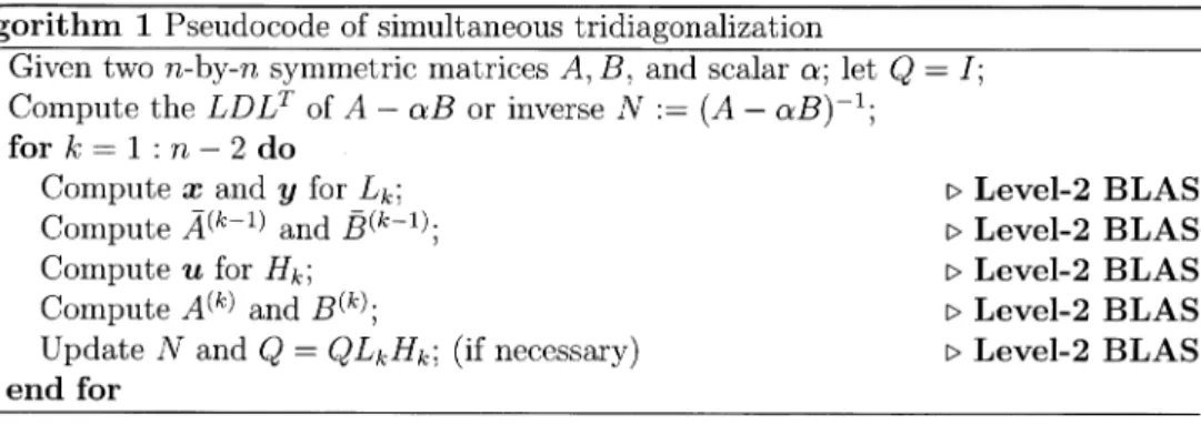
\overline{\frac{\mathrm{A}1\mathrm{g}\mathrm{o}\mathrm{r}\mathrm{i}\mathrm{t}\mathrm{h}\mathrm{m}1\mathrm{P}\mathrm{s}\mathrm{e}\mathrm{u}\mathrm{d}\mathrm{o}\mathrm{c}\mathrm{o}\mathrm{d}\mathrm{e}\mathrm{o}\mathrm{f}\mathrm{s}\mathrm{i}\mathrm{m}\mathrm{u}1\mathrm{t}\mathrm{a}\mathrm{n}\mathrm{e}\mathrm{o}\mathrm{u}\mathrm{s}\mathrm{t}\mathrm{r}\mathrm{i}\mathrm{d}\mathrm{i}\mathrm{a}\mathrm{g}\mathrm{o}\mathrm{n}\mathrm{a}1\mathrm{i}\mathrm{z}\mathrm{a}\mathrm{t}\mathrm{i}\mathrm{o}\mathrm{n}}{1:\mathrm{G}\mathrm{i}\mathrm{v}\mathrm{e}\mathrm{n}\mathrm{t}\mathrm{w}\mathrm{o}n-\mathrm{b}\mathrm{y}-n\mathrm{s}\mathrm{y}\mathrm{m}\mathrm{m}\mathrm{e}\mathrm{t}\mathrm{r}\mathrm{i}\mathrm{c}\mathrm{m}\mathrm{a}\mathrm{t}\mathrm{r}\mathrm{i}\mathrm{c}\mathrm{e}\mathrm{s}A,B,\mathrm{a}\mathrm{n}\mathrm{d}\mathrm{s}\mathrm{c}\mathrm{a}1\mathrm{a}\mathrm{r} $\alpha$;1\mathrm{e}\mathrm{t}Q=I;}}

2:

_Compute

the LD

L^{}

ofA- $\alpha$ B or inverse N

:=(A- $\alpha$ B)^{-1}

_;

3: for k=1 :n-2 do

4:

_Compute

x and _y for

L_{k}

_; \triangleright \mathrm{L}\mathrm{e}\mathrm{v}\mathrm{e}\mathrm{l}-2 BLAS

5:

_Compute

\overline{A}^{(k-1)}

and

\overline{B}^{(k-1)}

; \triangleright \mathrm{L}\mathrm{e}\mathrm{v}\mathrm{e}\mathrm{l}-2 BLAS

6:

_Compute

u for

H_{k}

_; \triangleright \mathrm{L}\mathrm{e}\mathrm{v}\mathrm{e}\mathrm{l}-2 BLAS

7:

_Compute

A^{(k)}

and

B^{(k)}

; \triangleright \mathrm{L}\mathrm{e}\mathrm{v}\mathrm{e}\mathrm{l}-2 BLAS

8:

_Update

N and

_{Q=QL_{k}H_{k}}

;

(if

necessary)

\triangleright \mathrm{L}\mathrm{e}\mathrm{v}\mathrm{e}\mathrm{l}-2 BLAS

9: end for

Weknow that almost all modern

_computers

have thestructure of_memory

_hierarchy.

Computation

timeofan

algorithm mainly depends

onthe arithmetic

operations

(FLOPs)

and data movement

_{(memory access).}

A basic rule for

_devising

fast

_algorithms

is to

reduce memory access as more as

possible.

The ratios of FLOPs _{to memory} access

corresponding

todifferent level

_operations

are

given

in Table 1.

Table 1: Ratios of arithmetic

_operations

_{to memory} access. Denote _$\alpha$,

$\beta$\in \mathbb{R},

_x,

y\in \mathbb{R}^{n}

and

_{A, B,}

C\in \mathbb{R}^{n\times n}.

\displaystyle \frac{\mathrm{F}\mathrm{L}\mathrm{O}\mathrm{P}\mathrm{s}\mathrm{m}\mathrm{e}\mathrm{m}\mathrm{o}\mathrm{r}\mathrm{y}\mathrm{a}\mathrm{c}\mathrm{c}\mathrm{e}\mathrm{s}\mathrm{s}\mathrm{R}\mathrm{a}\mathrm{t}\mathrm{i}\mathrm{o}}{y= $\alpha$ x+y(\mathrm{L}\mathrm{e}\mathrm{v}\mathrm{e}1-1)2n3n2/3}

y= $\alpha$ Ax+ $\beta$ y

(Leve1‐2)

2n^{2}

n^{2}

2

C= $\alpha$ AB+ $\beta$ C

(Leve1‐3)

2n^{3}

4n^{2}

_n/2

From Table

_1,

wesee that an

algorithm

that is ableto

_{implemented by higher}

level

BLAS

_operations

_maybe

show better

_performance,

which

inspires

us to extend the tridi‐

agonalization algorithm

and devise a new

algorithm

that can take

advantage

of the

Leve1‐3 BLAS

_operations.

3

An

_algorithm

for simultaneous band reduction

In this

section,

we extend the ideas in Section 2 and _propose an

algorithm

for simulta‐

neous band reduction. Similarto the simultaneous

_{tridiagonalization,}

the

_computations

of band reduction will be also divided two

_stages.

We first process

t(t :=(s-1)/2

hereafter)

steps

like the

_stage

1 of

_Algorithm

1 tomaket

_pairs

ofvectors collinear. Then

we continue to do t

_steps

like the

_stage

2 of

Algorithm

1 to eliminate the

_{off‐diagonal}

nonzeroentries for all

_|i-j|>t.

As there are different variants for simultaneous

tridiagonalization,

in what

_follows,

our

_strategy

of band reduction is

mainly

based on the first variant that _y= O. For

simplicity,

we take t=2 and discuss the two

_stages

of simultaneous band reduction as

Assuming

thattwo

_steps

of band reduction of A and B have been

_complete.

Matrices

A^{(1)}

and

B^{(1)}

obtained are as

follows,

3.1

_Stage

1: construct

matrix

_{L_{2}}

The aim of this

_stage

is to construct amatrix

L_{2}

which makes t

pairs

ofvectors corre‐

sponding

to

\overline{A}^{(1)}

:=L_{2}^{T}A^{(1)}L_{2}

and

\overline{B}^{(1)}

_{:=L_{2}^{T}B^{(1)}L_{2}}

arecollinear. When t=2, we can

construct

_{L_{2}}

as

follows,

The unknown entries of

L_{2}^{(1)}

and

L_{2}^{(2)}

aredetermined

by

the similar

_strategy

in section

2.1. Wenote that the unknown entries of

L_{2}^{(2)}

will be determined after that of

L_{2}^{(1)}.

Applying

L_{2}^{(1)}

and

L_{2}^{(2)}

to

A^{(1)}

_{successively,}

wecould obtain the

following

twomatrices

with thesame

_pattern,

_{respectively.}

Thenonzeroentries denoted

\mathrm{b}\mathrm{y}\otimes

arewhatwe care

about.

and

\displaystyle \overline{A}^{(1)}=L_{2}^{(2)T}\overline{A}^{(1)}L_{2}^{(2)}=(*** **** \otimes\otimes\bigotimes_{\otimes}^{\otimes***} \otimes\otimes\bigotimes_{\otimes}^{\bigotimes_{*}^{*}} \bigotimes_{*}^{\otimes}*** \bigotimes_{*}^{\otimes}*** \bigotimes_{*}^{\otimes}*** \bigotimes_{*}^{\otimes}***)

Similarto

\overline{A}^{(1)}

,we canalso obtain

\overline{B}^{(1)}

.

Congruent

transformations

by

L_{2}^{(1)}

make

\overline{A}^{(1)}(4

:

8,

3)

and

\overline{B}^{(1)}(4:8, 3)

be collinear.

_Congruent

transformations

_by

L_{2}^{(2)}

make

\overline{A}^{(1)}(5:8, 4)

and

_{B^{(1)}(5:8,4)-}

be collinear and

_keep

the

_collinearity

of

_{\overline{A}^{(1)}(4:8,3)}

and

_{\overline{B}^{(1)}(4:8,3)}

.

3.2

_Stage

2:

construct

matrix

_{H_{2}}

In this

_stage,

we eliminate nonzero entries of

\overline{A}^{(1)}

and

\overline{B}^{(1)}

in columns 3 and 4 for

the band form. We construct the matrix

H_{2}

as

follows,

a

product

of two Householder

matrices

H_{2}^{(1)}

and

H_{2}^{(2)},

where u_{4} and u_{3} can be determined

by

\overline{A}^{(1)}

(5

:

8,

3 :

4).

Then we can obtain

A^{(2)}=

H_{2}^{T}\overline{A}^{(1)}H_{2}

and

_{B^{(2)}=H_{2}^{T}\overline{B}^{(1)}H_{2}.}

As the

_product

of

H_{2}^{(1)}

and

H_{2}^{(2)}

can be

represented

as follows

by

the

_compact

WY

representation

[14],

H_{2}=\left(1 & 1 & 1 & 1 & I-VTV^{T}\right),

where V is a 4 \mathrm{x}2

matrix,

and T denotes a 2\times 2 _upper

triangular

matrix. In

practice,

sub‐matrices

A^{(2)}

₍₅

:

8,

5 :

8)

and

B^{(2)}(5

:

8,

5 : 8

)

can be

effectively computed by

this

representation,

Leve1‐3 BLASsuch as \mathrm{D}\mathrm{S}\mathrm{Y}\mathrm{R}2\mathrm{K}_, DSYMM canbe

employed.

We summarize discussion above and

_give

the

_pseudocode

of band reduction in

_Algo‐

rithm 2.

Remark 3.1. If s=3,

Algorithm

2 is consistent with the

Algorithm

1

corresponding

to

variant

_(i).

We note that the

_strategy

discussed in this section can be also

applied

to

\displaystyle \frac{\mathrm{A}1\mathrm{g}\mathrm{o}\mathrm{r}\mathrm{i}\mathrm{t}\mathrm{h}\mathrm{m}2\mathrm{P}\mathrm{s}\mathrm{e}\mathrm{u}\mathrm{d}\mathrm{o}\mathrm{c}\mathrm{o}\mathrm{d}\mathrm{e}\mathrm{o}\mathrm{f}\mathrm{b}\mathrm{a}\mathrm{n}\mathrm{d}\mathrm{r}\mathrm{e}\mathrm{d}\mathrm{u}\mathrm{c}\mathrm{t}\mathrm{i}\mathrm{o}\mathrm{n}}{1:\mathrm{G}\mathrm{i}\mathrm{v}\mathrm{e}\mathrm{n}\mathrm{s}\mathrm{y}\mathrm{m}\mathrm{m}\mathrm{e}\mathrm{t}\mathrm{r}\mathrm{i}\mathrm{c}\mathrm{m}\mathrm{a}\mathrm{t}\mathrm{r}\mathrm{i}\mathrm{c}\mathrm{e}\mathrm{s}A,B,Q=I\mathrm{a}\mathrm{n}\mathrm{d}\mathrm{s}\mathrm{c}\mathrm{a}\mathrm{l}\mathrm{a}\mathrm{r} $\alpha$;}

2: Given bandwidth s, let

t=(s-1)/2

;

3:

_Compute

the LD

L^{}

ofA- $\alpha$ B or inverse N

:=(A- $\alpha$ B)^{-1}

_; \trianglerightInverse

4: for

_{k=1:\displaystyle \mathrm{L}\frac{n-t}{t}\rfloor}

do

5: for

_i=(k-1)t+1

: kt do

6:

_Compute

_{x_{n-i}} for

L_{k}^{(i-(k-1)t)}

_; \triangleright \mathrm{L}\mathrm{e}\mathrm{v}\mathrm{e}\mathrm{l}-2 BLAS

7:

_Compute

\overline{A}^{(k)}(:, i)

and

_{\overline{B}^{(k)}(:, i)}

; \triangleright \mathrm{L}\mathrm{e}\mathrm{v}\mathrm{e}\mathrm{l}-2 BLAS

8:

_Update

N and

Q=QL_{k}^{(i-(k-1)t)}

;

(if

necessary)

\triangleright \mathrm{L}\mathrm{e}\mathrm{v}\mathrm{e}\mathrm{l}-2 BLAS

9: end for

10:

_Compute

the

_{QR decomposition}

of

_{\overline{A}(kt+1 : n, (k-1)t+1 : kt)}

and

_compact

_{WY‐representation}

of

_{H_{k}}

; \triangleright \mathrm{L}\mathrm{e}\mathrm{v}\mathrm{e}\mathrm{l}-2 BLAS

11:

_Compute

A^{(k)}=H_{k}^{T}A^{(k-1)}H_{k}

_; \triangleright \mathrm{L}\mathrm{e}\mathrm{v}\mathrm{e}\mathrm{l}-3 BLAS

12:

_Compute

B^{(k)}=H_{k}^{T}B^{(k-1)}H_{k}

_; \triangleright \mathrm{L}\mathrm{e}\mathrm{v}\mathrm{e}\mathrm{l}-3 BLAS

13:

_Update

N and

_{Q=QH_{k}}

;

(if necessary)

\triangleright \mathrm{L}\mathrm{e}\mathrm{v}\mathrm{e}\mathrm{l}-3 BLAS

14: end for

4

Numerical

_experiments

Inthis

_section,

we

give

somenumerical results to show the

_performance

of the

_proposed

algorithm.

We also

_apply

the

_algorithm

for

_{solving generalized}

shifted linear

_systems.

Test matriceswere initialized

by

random values andtwodifferent sizes

_{(n=1000, 3000)}

.

The

_computer

_{specifications}

are Red Hat

Linux,

AMD

Opteron(tm)

_processor, 2.5\mathrm{G}\mathrm{H}\mathrm{z}

(1 core)

with 32\mathrm{G}\mathrm{B} of RAM. The

_algorithm

was

implemented

inthe Fortran 90

language

and

_compiled

with ifort

_(ver.

_13.1.1)

_using

the Intel MKL for LAPACK and BLAS. In

the

_{implementation,}

we didnot

_compute

the

Q explicitly,

but the inverse of A- $\alpha$ B.

In

_Figure

_1,

we _compare the

computation

time of band reduction

corresponding

to

Algorithm

2withdifferent bandwidth. Weseethat the total

_computation

time isreduced

with

_greater

bandwidth.

_Compared

with s=3, the

algorithm

took less than half time

when s=17. In

Figure

2, symmetric

band linear

systems

Kx=bweresolved

by calling

the

_Lapack

function DGBSV. The

_computation

timealmost increased

_linearly

with the

increasing

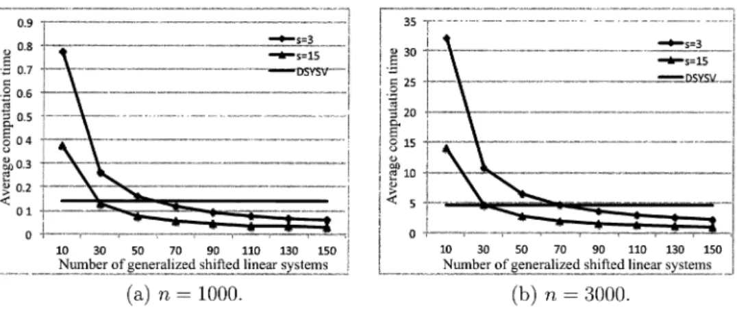
of bandwidth. We also

_computed

the solution of

_generalized

shifted linear

systems

(A+$\sigma$_{i}B)x=b

for i=1,

2,

..._,L

by using

band reduction and DGBSV. The

total

_computation

time is denoted

_by

_{T_{total} :=T_{bandreduction}+L\cdot T_{DGBSV}}

. In

Figure

3,

we show the _average

computation

time for one linear

_system,

i.e.,

T_{total}/L

.

Compared

to

_DSYSV,

band reduction shows its

_advantages

when the bandwidths and number of

shifted linear

_systems

L are

_greater.

5

Conclusions and future work

In this paper, we

proposed

an

algorithm

for simultaneous band reduction oftwo dense

symmetric

matrices.

_Although

our discussions are based on real‐valued

matrices,

the

algorithm

can be

easily

extended to

_{complex‐valued}

Hermitian matrices. We also _gave

(a)

n=1000.

_(b)

n=3000.

Figure

1:

_Computation

timeof band reduction

_{(in seconds)}

versus matrix bandwidth.

(a)

n=1000.

(

\mathrm{b}

)

n=3000.

Figure

2:

_Computation

time of band linear

_systems

_{(in seconds)}

versus matrix band‐

width.

(a)

n=1000.

(

\mathrm{b}

)

n=3000.

Figure

3:

_Average

_computation

time _per linear

_system

_{(in seconds)}

versus the number

width andan

application

of

solving generalized

shifted linear

_systems.

The

_topics,

suchas

other

_algorithms

for band

_reduction,

simultaneously

reduce band formto

_{tridiagonal form,}

accelerate the

_{computing using}

GPU

etc.,

will be considered as our future work.

Acknowledgments

This research was

partially supported by Strategic Programs

for Innovative Research

(SPIRE)

Field 5 (The

_origin

of matter’and the

_universe”,

_JST/CREST

_project

“Devel‐

opment

ofan

Eigen‐Supercomputing Engine using

aPost‐Petascale Hierarchical Model”’

and KAKENHI

_(Nos.

_25870099,

_25104701,

_25286097).

References

[1]

B.

_Adlerborn,

K. Dackland and B.

_Kagström,

Parallel and Blocked

_Algorithms

for Reduction ofa

Regular

Matrix Pairto

_{Hessenberg‐Triangular}

and Generalized

Schur

_Forms,

in

_Applied

Parallel

_Computing,

Lecture Notes in

_Comput.

Sci.

_2367,

Springer, Berlin, Heidelberg,

757-767(2006)

.

[2]

M.A.

_Brebner,

and J.

_{Grad, Eigenvalues}

ofAx = $\lambda$ Bx for Real

_Symmetric

Matrices

A and B

_{Computed by}

Reduction toa

Pseudosymmetric

Formand the HR_process,

Linear

_{Algebra Appl.,}

_43,

_99-118(1982)

.

[3]

C.H.

_Bischof,

B.

_Lang

and X.B.

_Sun,

A framework for

_symmetric

band

_reduction,

ACM Trans. Math.

_Software,

_{26(4), 581-601(2000)}

.

[4]

K. Dackland and B.

_Kagström,

Block

_algorithms

and software for reduction of a

regular

matrix

_pair

to

_generalized

Schur

_form,

ACM Trans. Math.

_Software,

_25(4),

425-454(1999)

.

[5]

L.

_Elsner,

A. Fasse and E.

_Langmann,

A

_{divide‐and‐conquer}

methodfor the

_tridiago‐

nal

_{generalized eigenvalue problem,}

J.

_{Comput. Appl. Math.,}

_86(1),

_{141-148(1997)}

.

[6]

S.D.

_Garvey,

F.

_Tisseur,

M.I.

_Friswell,

J.E.T.

_Penny

and U.

_Prells,

Simultaneous

tridiagonalization

of two

_{symmetric matrices,}

Int. J. Numer. Meth.

_Eng.,

_57(12),

1643-1660(2003)

.

[7]

B.

_Kagström,

D.

_Kressner,

E.S.

_{Quintana‐ortí}

and G.

_{Quintana‐ortí,}

Block

_algo‐

rithmsfor the reductionto

_{Hessenberg‐triangular}

form

_revisited,

BIT Numer.

_Math.,

48(3), 563-584(2008)

.

[8]

L.

_Kaufman,

An

_Algorithm

for the Banded

_Symmetric

Generalized Matrix

_Eigen‐

[9]

K.

_Li,

T.Y. Li and Z.

_Zeng,

An

_algorithm

for the

_generalized

_symmetric

_tridiagonal

eigenvalue problem,

Numer.

_Algorithms,

_{8(2), 269-291(1994)}

.

[10]

K.

_Li,

Durand‐Kerner

_{root‐finding}

method for the

_{generalized tridiagonal eigen‐}

problem,

Missouri J. Math.

_Sci.,

_33-43(1999)

.

[11]

R.S. Martin and J.H.

_Wilkinson,

Reduction of the

_symmetric

_eigenproblem

Ax =

$\lambda$ Bx and related

_problems

tostandard

_form,

Numer.

_Math.,

_{11(2), 99-110(1968)}

.

[12]

C.B. Moler and G.W.

_Stewart,

An

_algorithm

for

_generalized

matrix

_{eigenvalue prob‐}

Iems,

SIAM J. Numer.

Anal.,

10(2), 241-256(1973)

.

[13]

G. Peters and J.H.

_{Wilkinson, Eigenvalues}

of Ax = $\lambda$ Bx with band

_symmetric

A

and

_B,

_{Comput. J.,}

_{12(4), 398-404(1969)}

.

[14]

R. Schreiber and C. van

Loan,

A

storage‐efficient

WY

_{representation}

for

products

of householder

_{transformations,}

SIAMJ. Sci. Stat.

_Comput.,

_10(1),

_52-57(1989)

.

[15]

R.B.

_Sidje,

On the simultaneous

_{tridiagonalization}

oftwo

_symmetric

_matrices,

Nu‐

mer.

Math.,

118(3),

549-566(2011)

.

[16]

F.

_{Tisseur, Tridiagonal‐diagonal}

reduction of

_symmetric

indefinite

_pairs,

SIAM J.

Matrix Anal.

_Appl.,

_26(1),

_{215-232(2004)}

.

[17]

F.G. van

Zee,

R.A. van de

Geijn,

G.

Quintana‐ortí

and G.J.

Elizondo,

Families of

algorithms

for

_reducing

a matrix to condensed

form,

ACM Trans. Math.

Software,