Surface-links and marked graph diagrams (Intelligence of Low-dimensional Topology)

全文

(1)77. 数理解析研究所講究録第2004巻 2016年 77-88. Surface‐links and marked. Sang Department. surface‐link is. knot is of. Youl Lee. Mathematics, Pusan National University. Introduction. 1 A. of. graph diagrams. one. a. closed surface. smoothly embedded. in Euclidean. 4‐space \mathbb{R}^{4}. A surface‐. component surface‐link. A2‐sphere link is sometimes called a 2‐link. A2‐link component is called a 2‐knot. Two surface‐links \mathcal{L} and \mathcal{L}' in \mathbb{R}^{4} are equivalent if. a one. are ambient isotopic, that is, there is an orientation preserving homeomorphism \mathbb{R}^{4}\rightar ow \mathbb{R}^{4} such that h(\mathcal{L})=\mathcal{L}' or, equivalently, there exists a smooth family of diffeomorphisms f_{s} : \mathbb{R}^{4}\rightarrow \mathbb{R}^{4}(s\in[0,1]) such that f_{0}=\mathrm{i}\mathrm{d}_{\mathbb{R}^{4} the identity of \mathbb{R}^{4} and f_{1}(\mathcal{L})=\mathcal{L}' If each component \mathcal{K}_{i} of a surface‐link \mathcal{L}=\mathcal{K}_{1}\cup\cdots\cup \mathcal{K}_{ $\mu$}( $\mu$\geq 1) is oriented,. they h. :. ,. ,. .. then \mathcal{L} is called. an. oriented. h|_{\mathcal{L}. Two oriented surface‐links \mathcal{L} and \mathcal{L}'. surface‐link.. are. equivalent. \mathcal{L}\rightar ow \mathcal{L}' of h is also orientation preserving. A marked graph diagram is a link diagram in \mathbb{R}^{2} possibly with some 4‐valent vertices in which each 4‐valent vertex has a marker indicated by a small segment — S. J. K. Jr. and Yoshikawa introduced a method of surface‐links Lomonaco, presenting [15] [18] if the restriction. :. using marked graph diagrams. Indeed, every surface‐link is presented by a marked graph diagram (cf. [15, 18]) and such a presentation diagram is unique up to Yoshikawa moves (see Theorem 2.3). By using marked graph diagram presentation for surface‐links, some. properties and invariants of surface‐links were studied in [1, 2, 4, 6, 8, 9, 12, 13, 14, 16, 18]. In this short survey paper, we give a brief introduction to marked graph diagram presen‐ tation of surface‐links and a method of constructing ideal coset invariants for surface‐links introduced in [4, 14] by means of a polynomial invariant \ll\cdot\gg for marked graphs in \mathbb{R}^{3} defined by using a state‐sum model with classical link invariants as its state evaluation. Section 2 presents marked graph diagram presentation of surface‐links. Section 3 deals with the polynomial invariant \ll\cdot\gg for marked graphs in \mathbb{R}^{3} Section 4 discusses ideal .. coset invariants derived from the. polynomial. \ll\cdot\gg. .. An extended version of this paper. will be appear in elsewhere.. 2. Marked. A marked. graph. graph diagrams is. a. spatial graph G. of surface‐links. in. \mathbb{R}^{3} such that G is. a. finite. regular graph possibly. each v_{i} is a rigid vertex, i.e., we fix a sufficiently with 4‐valent vertices, say v_{1}, v_{2} , , v_{n} ; small rectangular neighborhood N_{i}\cong\{(x, y)\in \mathbb{R}^{2}|-1\leq x, y\leq 1\} , where v_{i} corresponds .. to the. .. .. origin and the edges incident to v_{i} are represented by x^{2}=y^{2} ; each v_{i} has a marker, on N_{i} given by \displaystyle \{(x, 0)\in \mathbb{R}^{2}|-\frac{1}{2}\leq x\leq\frac{1}{2}\} Two marked graphs are. which is the interval. ..

(2) 78. equivalent if they. are. ambient isotopic in \mathbb{R}^{3} with. keeping rectangular neighborhoods. and. markers. An orientation of in such. a. a. marked. graph G. is. choice of. a. an. orientation for each. \geq $\xi$ \ovalbox{\t smal REJ CT} Otherwise,. way that every vertex in G looks like. or. .. A marked. edge of G. graph. is said. it is said to be nonorientable. By an orientation. graph we mean an orientable marked graph with a fixed orientation. Two oriented marked graphs are equivalent if they are ambient isotopic in \mathbb{R}^{3} with keeping rectangular neighborhoods, orientation and markers. An oriented marked graph G in \mathbb{R}^{3} can be described as usual by a diagram D in \mathbb{R}^{2} which is an oriented link diagram in \mathbb{R}^{2} possibly with some marked 4‐valent vertices whose incident four edges have orientations illustrated as above, and is called an oriented marked graph diagram of G (cf. Figure 1). to be orientable if it admits an. oriented marked. ,. Figure. 1: Oriented marked. Two oriented marked. graphs. in. graph diagrams. graph diagrams. \mathbb{R}^{3} if and only if they. of oriented mark. are. and. in. a. nonorientable marked. graph diagram. \mathbb{R}^{2} represent equivalent oriented marked. transformed into each other. by. finite sequence (simply, oriented. a. preserving rigid 4‐regular spatial graph preserving RV4 moves) \mathrm{r}_{1}, $\Gamma$_{1}', $\Gamma$_{2}, $\Gamma$_{3}, $\Gamma$_{4}, $\Gamma$_{4}' and $\Gamma$_{5} shown in Figure 2, which consists Yoshikawa moves of type I (see Theorem 2.3). vertex. moves. mark. $\Gamma$_{1}. :. $\Gamma$ í. :. \vec{-}. $\Gamma$_{2}. :. \vec{-}. $\Gamma$_{3}. :. \leftarrow^{\rightarrow}. $\Gamma$_{4}. :. \leftarrow^{\vec{}}. $\Gamma$_{4}'. :. $\Gamma$_{5}. :. Figure. \backslash *_{-}t 2: Oriented mark. \leftarrow^{\vec{}}. \supset \supset \mathfrak{D}\mathrm{C}. /*-\sear ow\mathrm{t}_{\rangle}. preserving RV4. moves.

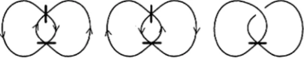
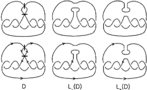
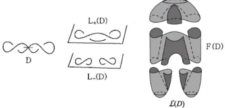
(3) 79. An unoriented marked. graph diagram. simply,. marked. graph diagram is a nonori‐ graph diagram in \mathbb{R}^{2} Two marked graph diagrams in \mathbb{R}^{2} represent equivalent marked graphs in \mathb {R}^{3} if and only if they are transformed into each other by a finite sequence of the moves $\Omega$_{1}, $\Omega$_{2}, $\Omega$_{3}, $\Omega$_{4}, $\Omega$_{4}' and $\Omega$_{5)} entable. or. or,. a. orientable but not oriented marked. an. .. where $\Omega$_{i} stands for the move $\Gamma$_{i} without orientation. For an (oriented) marked graph diagram D , let L_{-}(D) and link. diagrams. respectively,. obtained from D. illustrated in. as. by replacing. 3. We call. Figure. L_{+}(D). each marked vertex. L_{-}(D). and. be the. (oriented). \timeswith) (. L_{+}(D). and. ,. the negative resolution diagram D is. and the positive resolution of \mathrm{D} , respectively. An (oriented) marked graph admissible if both resolutions L_{-}(D) and L_{+}(D) are trivial link diagrams.. Figure Let D be Define. where. L_{-}(D). a. a. 3: Marked. graph diagrams. given admissible marked graph diagram with marked F(D)\subset \mathbb{R}^{3}\times[-1, 1] by. vertices v_{1} ,. .. .. .. ,. v_{n}.. surface. (\mathb{R}_t^{3},F(D)\cap mathb{R}_t^{3})=\left{\begin{ar y}{l (\mathb{R}^3,L_{+}(D)&\mathr {f}\mathr {o}\mathr {}0<t\leq1,\ (mathb{R}^3,L_{-}(D)\cup(bigcup_{i=1}^nB_{i})&\mathr {f}\mathr {o}\mathr {}t=0,\ (mathb{R}^3,L_{-}(D)&\mathr {f}\mathr {o}\mathr {}-1\leqt<0, \end{ar y}\ight.. \mathb {R}_{t}^{3} :=\{(x_{1}, x_{2}, X3, x_{4})\in \mathbb{R}^{4}|x_{4}=t\}. surface. and their resolutions. at each marked vertex v_{i}. as. and. illustrated in. B_{i}(1\leq i\leq n) Figure. 4.. associated with D.. \rightarrow. Figure. When D is entation of D. \displaystle\frac{\mathrm{B}_\mathrm{i}. 4: A band attached to. is. a. We call. band attached to. F(D). the proper. \mathrm{L}-(\mathrm{D})\cup\{\mathrm{B}_{\mathrm{i} \}. L_{-}(D). at v_{i}. oriented, L_{-}(D) and L_{+}(D) have the orientations induced from the ori‐ (cf. Figure 3), We assume that the proper surface F(D) is oriented so. that the induced orientation. on. L_{+}(D)=\partial F(D)\cap \mathbb{R}_{1}^{3}. matches the orientation of. L_{+}(D). ..

(4) 80. F(D) by attaching trivial disks in resulting (oriented) \mathbb{R}^{3}\times(-\infty 1]. \mathbb{R}^{3}\times[1, \infty) surface‐link by \mathcal{L}(D) and call it the (oriented) surface‐link associated with D It is well known that the isotopy type of \mathcal{L}(D) does not depend on the choices of trivial disks (cf. Figure 5 shows a schematic picture of the surface‐link \mathcal{L}(D) associated with a [5, 7 Since D is. admissible,. we can. obtain. surface‐link from. a. and another trivial disks in. We denote the. ,. .. ,. marked. graph diagram D.. \mathrm{D}. \mathrm{L}_{-}(\mathrm{D}). \mathcal{L}(D) Figure. Definition 2.1. Let \mathcal{L} be. (oriented) surface‐link \mathcal{L}(D). by. marked. an. Let D be. presented by From. now. (oriented). \mathbb{R}^{3}\times \mathbb{R}. ambient. an. in \mathbb{R}^{4}.. we. (oriented). show that any. be deformed into. all critical. points. in such are. a. a. graph diagram. .. marked. (oriented). We say that \mathcal{L} is isotopic to the. graph diagram.. surface‐link is. D. presented. (oriented). By definition, \mathcal{L}(D). presented by. an. is. admissible. [7] that any surface‐link \mathcal{L} in \mathbb{R}^{4}= called a hyperbolic splitting of \mathcal{L} by an. is well known. surface‐link L' ,. ,. projection p:\mathcal{L}'\rightarrow \mathbb{R} satisfies the followings:. non‐degenerate,. all the index 1 critical. (minimal points). points (saddle points). all the index 2 critical points a. marked. D if \mathcal{L} is ambient. way that the. all the index 0 critical points. Let \mathcal{L} be. a. surface‐link in \mathb {R}^{4}. (oriented). graph diagram. It. isotopy of \mathbb{R}^{4}. associated with. graph diagram. admissible. marked. can. an. D. on,. \mathcal{L}(D). 5: A surface‐link. are. (maximal points). surface‐link and let \mathcal{L}' be. a. \mathcal{L} Ó =\mathcal{L}. \mathb {R}_{0}^{3}. are. in. are. in. \mathbb{R}_{-1}^{3},. \mathb {R}_{0}^{3}, in. \mathb {R}_{1}^{3}.. hyperbolic splitting of \mathcal{L} Then the .. . \cap \mathb {R}_{0}^{3}. cross‐section. at t=0. We give a marker at each 4‐valent vertex (saddle point opens up above as illustrated in Figure 6. When \mathcal{L} is an oriented surface‐link, we choose an orientation for each edge of \mathcal{L} Ó so that it coincides with the induced orientation on the boundary of \mathcal{L}'\cap \mathbb{R}^{3}\times(-\infty, 0 ] by is. a. spatial. point). 4‐valent. regular graph. in. that indicates how the saddle. ..

(5) 81. \times Figure. 6: A marker at. a. 4‐valent vertex. The resulting (oriented) marked graph presenting \mathcal{L} A diagram D of the (oriented) marked graph G is clearly admissible, and is called an (oriented) marked graph diagram or (oriented) ch‐diagram presenting \mathcal{L} In conclusion, we state the followings.. the orientation of \mathcal{L}' inherited from the orientation of \mathcal{L} G. graph. :=. \mathcal{L} Ó is called. an. (oriented). .. marked. .. .. Theorem 2.2 there is. (2). an. Let \mathcal{L} be. ([7]). (1) Let D be an admissible (oriented) (oriented) surface‐link \mathcal{L} presented by D.. an. (oriented). graph diagram. surface‐link. Then there is. an. marked. admissible. presenting \mathcal{L}.. D. ([9, 10,. graph diagram.. (oriented). Then. marked. (1) Two oriented marked graph diagrams present the same only if they are transformed into each other by a finite sequence mark preserving RV4 moves in Figure 2, called oriented Yoshikawa moves of oriented Yoshikawa moves of type II in Figure 7.. Theorem 2.3. 17. oriented surface‐link if and. of oriented. type I and ,. $\Gamma$_{6}. :. \underline{\rightarrow}. \supset. $\Gamma$_{6}'. :. \leftarrow^{\vec{}}. \supset. $\Gamma$_{7}. $\Gamma$_{8}. \vec{-}. :. :. Figure. 7: Oriented Yoshikawa. moves. of type II. (2). Two unoriented marked graph diagrams present the same unoriented surface‐link only if they are transformed into each other by a finite sequence of unoriented mark preserving RV4 moves $\Omega$_{1}, $\Omega$_{2}, $\Omega$_{3}, $\Omega$_{4}, $\Omega$_{4}', $\Omega$_{5} called unoriented Yoshikawa moves of type I and unoriented Yoshikawa moves of type II $\Omega$_{6}, $\Omega$_{6)}'$\Omega$_{7} and $\Omega$_{8} where $\Omega$_{i} stands for the move $\Gamma$_{i} without orientation. if and. ,. ,. ,.

(6) 82. invariants for marked. Polynomial. 3. graphs. in \mathbb{R}^{3} via classical. link invariants Let R be. a. commutative. the additive. ring with. identity. 0 and the. multiplicative identity. 1 and let. [ ] : {classical be. a regular $\delta$\in R,. or an. ambient. isotopy. knots and links in. \mathb {R}^{3} } \rightarrow R. invariant such that for. a. unit $\alpha$\in R and. [_{/}^{\backslash }<)]= $\alpha$[)], [_{/}^{\backslash } [K\mathrm{O}]= $\delta$[K]. an. (3.1). .. (3.2). ,. where. K\mathrm{O}. denotes any addition of. a. disjoint. circle. \mathrm{O}. to. a. element. classical knot. or. link. diagram. K. For in. a. R[x, y]. given marked graph diagram D let [[D]](x, y) ( [ \mathrm{D}] for short) be ,. defined. (L1) [[D]]=[D]. (L2). by. the. if D is. a. following link. a. polynomial. two rules:. diagram,. [ \rangle\langle] =[\left\{\begin{ar ay}{l} \\. \end{ar ay}\right\}]x+[[)(] y.. When D is. oriented marked. an. links, then [[D]]. (L1) [[D]]=[D]. graph diagram. is defined. by. if D is. oriented link. an. (L2). [ \S $\xi$] =[\left\{\begin{ar ay}{l} \aleph-\near ow\ \near ow\ap rox \end{ar ay}\right\}]x+[ ) $\zeta$] y). (L3). =[\left\{ begin{ar ay}{l} \backslash \rightar ow\ )= \end{ar ay}\right\}]_{X}+[ 2\backslash \upar ow] y.. Let. and. the rules:. [. ]. is. an. invariant for oriented. diagram,. D=D_{1}\cup\cdots\cup D_{m} be an oriented link diagram and let w(D_{i}) be the usual writhe D_{i} The self‐writhe sw(D) of D is defined to be the sum. of the component. .. sw(D)=\displaystyle \sum_{i=1}^{m}w(D_{i}) Now let D be. a. marked. graph diagram. We. .. choose. an. arbitrary. orientation for each. component of L_{+}(D) and L_{-}(D) When D is oriented, we choose orientations for L_{+}(D) and L_{-}(D) induced from the orientation of D We define the self‐writhe sw(D) of D by .. .. sw(D)=\displaystyle \frac{sw(L_{+}(D) +sw(L_{-}(D) }{2}, where. sw(L_{+}(D)). and. sw(L_{-}(D)) are independent L_{+}(D) and L_{-}(D). the writhe of each component of tation for the component.. of the choice of orientations because is. independent of. the choice of orien‐.

(7) 83. It is noted that the self‐writhe move. $\Omega$_{1}. .. For. $\Omega$_{1}. Definition 3.1. Let D be. ( \ll D\gg. for. sw(D). and its mirror move,. short). an. to be the. by. is invariant under Yoshikawa. we. (oriented). marked. polynomial. moves. except the. have. graph diagram. We define \ll D\gg(x, y) x and y with coefficients in R given. in variables. \ll D\gg=$\alpha$^{-sw(D)}[[D]](x, y)\in R[x, y]. Let D be. an. (oriented). each marked vertex in D. .. marked Let. diagram.. S(D). A state of D is. assignment of T_{\infty}. an. be the set of all states of D. .. For each state. or. T_{0}. to. $\sigma$\in \mathcal{S}(D). ,. D_{ $\sigma$} denote the (oriented) link diagram obtained from D by replacing marked vertices of D with two trivial 2‐tangles according to the assignment T_{\infty} or T_{0} by the state $\sigma$ : let. \rangle\langle T_{\infty}\rightar ow, \rangle\langle T_{0}\rightar ow)(\cdot. 3_{T_{\infty} $\xi$\rightar ow\ap rox\mapsto, \S_{T_{0} $\xi$\rightar ow \mathrm{j} $\zeta$,. \geq\leqT_{\infty}\rightar ow\infty\mapsto 3_{T_{0} \leq\rightar ow)\upar ow. . Then \ll D\gg has the. following. state‐sum. formula:. \displaystyle \l D\g =$\alpha$^{-sw(D)}\sum_{ $\sigma$\in \mathcal{S}(D)}[D_{ $\sigma$}]x^{ $\sigma$(\infty)}y^{ $\sigma$(0)}, where. $\sigma$(\infty). and. respectively.. Theorem 3.2. (oriented). $\sigma$(0). ([14]).. marked. denote the numbers of the. Let G be. graph diagram. an. of G. assignment T_{\infty} and T_{0} of the. state $\sigma$,. marked graph in \mathbb{R}^{3} and let D be an given regular or ambient isotopy invariant. (oriented) .. For any. [ ] : {classical (oriented). links in. \mathb {R}^{3} } \rightarrow R. properties (3.1) and (3.2), the polynomial \ll D\gg is an invariant for moves of type I, and therefore it is an invariant of the (oriented) (oriented) marked graph G in \mathbb{R}^{3}.. satisfying. the. Yoshikawa. Ideal coset invariants for surface‐links. 4. An oriented. ‐tangle diagram (n\geq 1) is an oriented link diagram T in the rectangle in \mathbb{R}^{2} such that T transversely intersect with (0,1)\times\{0\} and (0,1)\times\{1\} distinct points, respectively, called the endpoints of T. n. I^{2}=[0, 1]\times[0 1 ] ,. in. n.

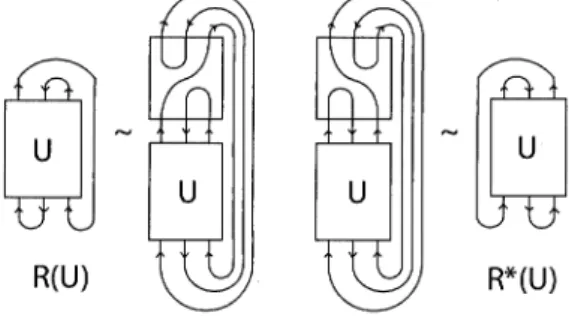
(8) 84. Let. T_{3}^{\mathrm{o}\mathrm{r}\mathrm{i}. and. T_{4}^{\mathrm{o}\mathrm{r}\mathrm{i}. orientations of the orientations. as. denote the set of all oriented 3‐ and. arcs. shown in. 4‐tangle diagrams such that tangles intersecting the boundary of I^{2} coincide with (a) and (b) of Figure 8, respectively.. of the. (a) Figure For. U\in T_{3}^{\mathrm{o}\mathrm{r}\mathrm{i}. diagrams. and. V\in T_{4}^{\mathrm{o}\mathrm{r}\mathrm{i}. obtained from the. Figure. ,. (b). 8: Boundaries of. let. 3, 4‐tangle diagrams. R(U) R^{*}(U) S(V) ,. tangles. 9:. the the. ,. U and V. Closing operations. S^{*}(V). and. denote the oriented link. shown in. by closing. as. R and R^{*} of. a. 3‐tangle. U. a. 4‐tangle. V. Figures. 9 and 10.. \mathrm{S}(\mathrm{V}) \mathrm{S}^{*}(\mathrm{V}) Figure. 10:. Closing operations. S and S^{*} of. T_{3} and T_{4} denote the set of all 3‐ and 4‐tangle diagrams without orientations, respectively. For U\in T_{3} and V\in T_{4} let R(U) R^{*}(U) S(V) and S^{*}(V) be the link diagrams obtained by the same way as above forgetting orientations. Let. ,. ,. ,.

(9) 85. ([4]).. Definition 4.1. For any. given regular. ambient. or. [ ] : {classical (oriented) satisfying. links in. invariant. isotopy. \mathb {R}^{3} } \rightarrow R. properties (3.1) and (3.2), the [ ] obstruction ideal (or simply, [ ] ideal) R[x, y] generated by the polynomials in R[x, y] :. the. I. is defined to be the ideal of. P_{1}= $\delta$ x+y-1,. P_{2}=x+ $\delta$ y-1,. P_{U}=([R(U)]-[R^{*}(U)])xy, U\in T_{3}(T_{3}^{\mathrm{o}\mathrm{r}\mathrm{i}}) P_{V}=([S(V)]-[S^{*}(V)])xy, V\in T_{3}(T_{4}^{\mathrm{o}\mathrm{r}\mathrm{i}}) Theorem 4.2. ([4]).. The map. {(oriented). :. defined. by. for any. (oriented). ,. .. marked. graph diagrams}. \rightarrow R[x, y]/I. \overline{[]}(D)=\overline{[D]}:=\ll D\gg+I marked. Remark 4.3. Let F be. graph diagram. an. completely determined by i.e., I=<p_{1}, p_{2} p_{r}>. .. .. .. an. extension field of R. I is. ,. D is. a. .. finite number of. invariant for. (oriented). surface‐links.. By Hilbert Basis Theorem, the [ ] polynomials in F[x, y] say p_{1}, p_{2} ,. ,. .. ideal .. .. ,. p_{r},. ,. In the rest of the paper,. give the ideals of Kauffman bracket for unoriented links tangled trivalent graphs [11] and corresponding ideal coset invariants for unoriented surface‐links and oriented surface‐links, respectively. For more details, we refer to [3, 4, 14]. and. we. Kuperbergs quantum A_{2}. Let K be. a. knot. link. or. bracket for. diagram.. \langle K\}=\{K\rangle(A)\in R=\mathbb{Z}[A, A^{-1}] (B1) \langle \mathrm{O})=1, (B2) \{\mathrm{O}K'\rangle= $\delta$\langle K'\rangle (B3) where. ,. Kauffman bracket of K by the following rules:. is. a. Laurent. polynomial. $\delta$=-A^{2}-A^{-2},. where. \{/\backslash _{\backslash }\rangle=A\langle)(\rangle+A^{-1}\langle\rangle, \mathrm{O}K'. move. disjoint circle \mathrm{O} to a knot or link diagram K'. polynomial is invariant under Reidemeister moves except. denotes any addition of. Note that the Kauffman bracket. the. The. defined. $\Omega$_{1} and for $\alpha$=-A^{3}. ,. we. a. have. \langle\grave{/}0\rangle= $\alpha$\langle)\rangle, \langle\infty_{/}\rangle=$\alpha$^{-1}\langle)\rangle. Then the. polynomial \ll D\gg=\ll D\gg(A, x, y). in Definition 3.1 is. \ll D\gg=(-A^{3})^{-sw(D)}[[D]](A, x, y). =(-A^{3})^{-sw(D)}\displaystyle\sum_{$\sigma$\in\mathcal{S}(D)}x^{$\sigma$(\infty)}y^{$\sigma$(0)}\langleD_{$\sigma$}\rangle.. given by.

(10) 86. Theorem 4.4. The Kauffman bracket ideal I is the ideal of. \mathbb{Z}[A, A^{-1}, x, y] generated by. (-A^{2}-A^{-2})x+y-1, x+(-A^{2}-A^{-2})y-1, (A^{8}+A^{4}+1)xy. Moreover,. the map. :. \overline{\langle D\}}=\ll D\gg+I. {marked graph diagrams} \rightarrow \mathbb{Z}[A, A^{-1}, x, y]/I. for any marked. graph diagram. D is. an. defined. by. invariant for unoriented. surface‐links.. given oriented marked graph diagram D let \ll D\gg denote the polynomial \mathbb{Z}[a, a^{-1}, x, y] defined by the following recursive rules: For any. in. ,. (1). \ll $\Theta$\gg=1.. (2). If D and D' moves. $\Gamma$_{1}. ,. are. $\Gamma$ í,. two oriented marked. $\Gamma$_{2}, $\Gamma$_{3}, $\Gamma$_{4}, $\Gamma$_{4}'. ,. and. $\Gamma$_{5},. graph diagrams. related. (3). \ll D\sqcup $\Theta$\gg=(a^{-6}+1+a^{6})\ll D\gg.. (4). \ll\S $\xi$\gg=x\ll\nearrow\approx\aleph_{-}/\gg+y\ll) $\zeta$\gg.. (5). a^{-9}\l \nearrow^{\nwarrow\backslash }\gg-a^{9}\l \backslash _{/}^{\nearrow}\gg=(a^{-3}-a^{3})\l \backslash ,1\gg.. Theorem 4.5. Let I be the ideal of. by. oriented Yoshikawa. then \ll D\gg=\ll D'\gg.. \mathbb{Z}[a, a^{-1}, x, y] generated by. (a^{-6}+1+a^{6})x+y-1, x+(a^{-6}+1+a^{6})y-1, (a^{12}+1)(a^{6}+1)^{2}xy.. \overline{\{\rangle}_{A_{2} {oriented marked graph diagrams} \rightarrow \mathbb{Z}[a, a^{-1}, x, y]/I defined \overline{\langle D\rangle}_{A_{2}}=\ll D\gg+I for any oriented marked graph diagram D is invariant for. Then the map. by. :. an. oriented surface‐links.. We remark that the ideal I of. \mathbb{Z}[a, a^{-1}, x, y]. in Theorem 4.5 is. actually. the ideal of Ku‐. \overline{\{\rangle}_{A_{2}. is the corresponding bracket for oriented links and the map ideal coset invariant for oriented surface‐links (cf. [3, 11 We close this section with the. perbergs quantum A_{2}. following:. Question. 4.6. Is there. a. classical link invariant. [ ]. such that the. [ ]. ideal is trivial?. Acknowlegement This work. was. supported by. Program through the National Re‐ Ministry of Education, Science and. Basic Science Research. (NRF) Technology (2013\mathrm{R}\mathrm{I}\mathrm{A}\mathrm{I}\mathrm{A}2012446) search Foundation of Korea. .. funded. by. the.

(11) 87. References. [1]. S. Ashihara, Calculating the fundamental biquandles of surface links from their diagrams. J. Knot Theory Ramifications 21(2012), no. 10, 1250102 (23 pages).. [2]. Y.. ch‐. Joung, S. Kamada and S. Y. Lee, Applying Lipsons state models to marked graph diagrams of surface‐links, J. Knot Theory Ramifications 24 (2015), no. 10, 1540003. (18 pages).. Joung, S. Kamada, A. Kawauchi and S. Y. Lee, Polynomial of an oriented surface‐ diagram via quantum A_{2} invariant, arXiv:1602.01558.. [3]. Y.. [4]. Y.. [5]. S. Kamada, Braid and Knot Theory in dimension Four, Mathematical Surveys and Monographs 95, American Mathematical Society, Providence, RI, 2002.. [6]. link. Joung, J. Kim and S. Y. Lee, Ideal coset invariants for surface‐links Theory Ramifications 22 (2013), no. 9, 1350052 (25 pages).. [8]. 10, 1540010 (35 pages).. A. Kawauchi, T. Shibuya and S. Suzuki, Descriptions on surfaces in Normal forms, Math. Sem. Notes Kobe Univ. 10 (1982), 75‐125. J.. Kim,. Y.. [11]. and S. Y.. four‐space, I;. Lee, On the Alexander biquandles of oriented surface‐ J. Knot Theory Ramifications 23 (2014), no. 7,. graph diagrams,. (26 pages).. J. Kim, Y. Joung and S. Y. Lee, On generating sets of Yoshikawa graph diagrams of surface‐links, J. Knot Theory Ramifications. moves. 24. (21 pages).. for marked. (2015),. no.. 4,. C. Kearton and V. Kurlin, All 2‐dimensional links in 4‐space live inside a universal polyhedron, Algebraic & Geometric Topology 8 (2008), 1223‐1247.. 3‐dimensional. G. 5. [12]. Joung. links via marked. 1550018. [10]. ,. S. Kamada, J. Kim and S. Y. Lee, Computations of quandle cocycle invariants of using marked graph diagrams, J. Knot Theory Ramifications 24 (2015),. 1460007. [9]. \mathbb{R}^{4} J. Knot. surface‐links no.. [7]. in. Kuperberg, The Quantum G_{2} no. 1, 61‐85.. link. invariant, International Jounal of Mathematics. (1994),. Lee, Invariants of surface‐links in \mathbb{R}^{4} via classical link invariants. Intelligence of topology 2006, pp. 189‐196, Ser. Knots Everything, 40, World Sci. Publ., Hackensack, NJ, 2007. S. Y.. low dimensional. [13]. S. Y. Lee, Invariants of surface‐links in \mathb {R}^{4} via skein relation, J. Knot fications 17 (2008), no.4, 439‐469.. [14]. S. Y. Lee, Towards invariants of surfaces in 4‐space via classical link invariants, Trans. Amer. Math. Soc. 361 (2009), no. 1, 237‐265.. [15]. S. J. Lomonaco, Jr., The homotopy groups of knots I. How to compute the 2‐type, Pacific J. Math. 95 (1981), no. 2, 349‐390.. Theory. Rami‐. algebraic.

(12) 88. [16]. M. Soma, Surface‐links with square‐type ch‐graphs, Proceedings of the First Joint Japan‐Mexico Meeting in Topology (Morelia, 1999), Topology Appl. 121 (2002), 231‐ 246.. [17] [18]. F. J.. Swenton, On a calculus for 2‐knots and Ramifications 10 (2001), no. 8, 1133‐1141.. K. no.. Yoshikawa, An 3, 497‐522.. Department. enumeration of surfaces in. of Mathematics. Pusan National. University. Busan 46241. KOREA \mathrm{E} ‐mail address:. [email protected]. surfaces in. 4‐space, J. Knot Theory. four‐space, Osaka. J. Math. 31. (1994),.

(13)