Numerical methods of calculating projection to positive eigenspace (Quantum Statistical Inference and Geometric Structure)

Numerical

methods

of

calculating

projection

to

positive

eigenspace*1

大阪大学基礎工学研究科 田中冬彦

Fuyuhiko Tanaka

Graduate

School

ofEngineering Science Osaka University

Abstract

Recently, Sakashita andNagaoka presented their researchon numerical

sim-ulatipn of asymptotic methods in quantum statistics. Their method heavily

depends on accurate calculation of all the eigenvalues and eigenvectors of a

hugeHermitianmatrix. However, onlyaprojectionoperatortothe eigenspaee

corresponding to positive eigenvalues is necessary. We propose two different

numerical methods, both of which avoid numerical diagonalization.

1

Basic

Motivation

Recently, Sakashita and Nagaoka [9] has worked for numerical simulation of

asymp-totic methods in quantum statistics. Their method heavily depends on accurate

calculation of all the eigenvalues and eigenvectors of

$\{\rho^{\bigotimes_{1}n}-k\rho_{2}^{\otimes n}>0\}$, (1)

where $n$ is sufficiently large integer, $k$ is a real constant, and

$\rho_{1}$ and $\rho_{2}$

are

density

matrices in the two-dimensional Hilbert space. The notation $\{X >0\}$ for a given Hermitian matrix $X$ is defined by

$\{X>0\}:=a:\sum_{\lambda_{a}\in\sigma(X)}, \lambda_{a}>0^{E_{a}}$’

where$\sigma(X)$ denotesthe set ofeigenvalues (spectrum) of$X$and$E_{a}$ isaprojection

oper-ator corresponding to the eigenvalue $\lambda_{a}$

.

Other projection operators,

$\{X<0\},$ $\{X=$

$*1$

$0\}$

are

also defined in the

same manner.

The above projection operator (1) is indeed the quantum Neyman-Pearson test [4] for $\rho_{1}^{\otimes n}$ vs $\rho_{2}^{\otimes n}(k$ is determined according to the significance level Asymptotic behavior of some quantities derived from (1) has theoretical importance [6, 3, 5]. However,

our

proposed methods

are

very general and the author believes that they

are

important apart from quantum statistical significance.

Efficient computation of all the eigenvalues and eigenvectors

of a

huge but

struc-tured Hermitianmatrix$X$isthe

essence

ofthe previousresult [9]. However,

a

general-purpose method (diagonalization of

a

matrix)

was

applied to numerical computation

ofthe projection operator $\{X>0\}$ while not eigenvalues themselves but their signs

are

necessary. Thus, a basic question arises: Is there any other numerical method

comparable to the previous approach? Since the workshop,

some

discussions with

Sakashita have continued and finally

we

obtain two numerical methods of calculating $\{X >0\}$

.

Both

1nethods

avoid the numerical diagonalization of

a

Hermitian matrix to compute the projection operator.

2

Problem Setting

Suppose that a Hermitian

_matrix

$X$ in

a

$d$-dimensional complex vector space is

given. $(d is$ assumed $to be$ very large, $say, d=10^{6}.)$ _Our

purpose here

_is to propose

a

numerical method of computing projection operators without numerical diagonal-ization.

$\{X>0\}, \{X<0\}, \{X=0\}.$

We obtain two methods in the present article.

(i) Monte Carlo optimization (ii) Topological Method

Monte Carlo optimization is

one

of the most

common

optimization methods (See,

e.g., Robert and Casella [8]). Topological Method

uses

the stability of some points in

a

discrete-time dynamical system (See, e.g., Guckenheimer and Holmes [1] for dynamical systems). _{The latter method is developed by the author in order to deal}

with

our

problem.

3

Monte Carlo optimization

The first method applies the well-known optimization technique to

our

specific

problem. _{The basic idea is} very simple. We construct the objective function

so

that its maximizer is the desired projection $\{X >0\}$

.

Our method uses

some

_results in

classical and quantum hypothesis testing for simple hypotheses (See, e.g., Hayashi [2]

for basic notations and terminology).

Definition 1. Let $M:=\{M_{x}\}_{x\in \mathcal{X}}$ denote

a finite-valued

POVM $(|\mathcal{X}|<\infty)$

.

The set of test with $M$ is defined _by

$\mathcal{P}_{M}:=\{T=\sum_{x}\phi(x)M_{x}:0\leq\phi(x)\leq 1, \forall x\in \mathcal{X}\}$

and the whole set of test is defined by

$P_{full}:=\{T:0\leq T\leq I\}.$

(By definition $\mathcal{P}_{M}\subset \mathcal{P}_{full}.$)

It is easy to seethat both $\mathcal{P}_{M}$ and $\mathcal{P}_{full}$

are

closed (compact) and

convex.

We give

Forgeneral algorithm,

we can

select the candidatedistribution$\mu(U)$ tobe

indepen-dent of the current $M^{(n)}$

.

_{Practically speaking, it is inefficient and it would be faster}

to generate $U$ accordingto the current $M^{(n)}$ if

we

assume

some

_conditions

on

$X.$

It is easily

seen

that $\sup\{RTX : T\in \mathcal{P}\}$ is achieved when the

subset

$\mathcal{P}\subseteq \mathcal{P}_{full}$ is

compact. In order to understand the above algorithm,

we

need three lemmas (those

are easy to prove, thus, proofs are omitted

Lemma 1. Let $X$ be a Hermitianmatrix and $M=\{M_{x}\}_{x\in \mathcal{X}}$ be

a

POVM. Then

$\tilde{M}:=\sum_{x:TrXM_{x}>0}M_{x}$

achieves the following maximum.

The above result is anotherformof the result inclassicalBayesian hypothesis testing (See, e.g., Chap.5 in Robert [7] for Bayesian testing).

Now

we

define

$E_{U}:=\{UE_{1}U^{*}, . . . , UE_{d}U^{*}\},$

$\tilde{E}_{U}:=\arg\max\{TxTX:T\in \mathcal{P}_{E_{U}}\}$

for every unitary matrix $U\in \mathcal{U}$

.

In particular, the

following holds.

Lemma 2. For

a

standard PVM $E$ fixed,

$\mathcal{P}_{full}=\overline{co\{\mathcal{P}_{E_{U}}:U\in \mathcal{U}\}},$

where $co\{A\}$ denotes the closed

convex

_{hull of}a subset $A\subset \mathcal{P}_{full}$ and $\mathcal{U}$ denotes the

whole set ofunitary matrices.

For

a

pair of

subsets

satisfying $\mathcal{P}_{1}\underline{\subseteq}\mathcal{P}_{2},$

max{TrTX:

$T\in \mathcal{P}_{1}$

}

$\leq\max\{hTX_{\dot{\iota}}T\in \mathcal{P}_{2}\}$

holds. Using this monotonicity and the above Lemma 1 and Lemma 2,

we

easily obtain the following lemma, which is essential to

our

algorithm.

Lemma 3. For

a

standard PVM $E$ fixed, _the following _holds.

$\{X>0\}=\max\{$

TrTX

: $T\in \mathcal{P}_{full}\}$

$= \max\{\max\{$

TrTX

: $T\in \mathcal{P}_{E_{U}}\}:U\in \mathcal{U}\}$ $= \max\{h\tilde{E}_{U}X:U\in \mathcal{U}\}$

Clearly the last equality in Lemma 3

assures

the validity of our algorithm. For

a

sufficiently large $n,$ $M^{(n)}\approx\{X>0\}$

.

The projection to negative eigenspace _$\{X<0\}$

4

Topological

Method

First we deal with exceptional

cases

whererankX $=1$

.

In

numerical

calculation

we

do not have this information on X. $($Again, _$we$ emphasize that $X is a$ huge matrix.$)$

Without diagonalization and knowing eigenvalues,

we

can

decide whether rankX is equal to

one or

not by calculating $RX^{2}$ _and $(^{r}RX)^{2}$

.

When $X$ is

a

Hermitian matrix,

$hX^{2}\geq(RX)^{2}$ holds. In particular, rankX $=1$ if and only if Tr$X^{2}=(hX)^{2}$ and

$X\neq 0.$

Ifwe know rankX $=1$_{, then dividing} $X$ by the scalar $TrX$ _yields

$\{X>0\}=\{\begin{array}{ll}\frac{1}{TrX}X, X>0,0, X<0,\end{array}$

$\{X<0\}=\{\begin{array}{ll}0, X>0,\frac{1}{TrX}X, X<0,\end{array}$

$\{X=0\}=I-\{X>0\}-\{X<0\}.$

Now

we

assume

that rankX $\geq 2$ and present

our

main result. In this case,

we

may consider the maximum of the absolute eigenvalue is smaller than

one

for simplicity. Indeed $\Vert X\Vert_{2}$ $:=\sqrt{hX^{2}}>\Vert X\Vert_{\infty}$ when rankX $\geq 2$ and \’if

we

take $Y$ $:=X/\Vert X\Vert_{2}$

then $\{Y>0\}=\{X>0\}$ holds.

Our main result is due tothe following elementaryresult in

a

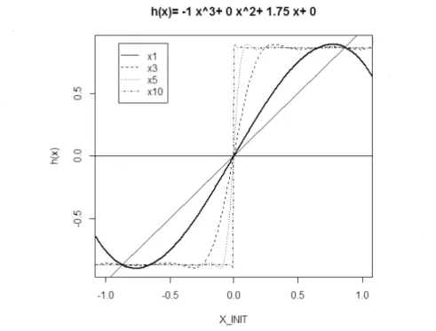
discrete-time dynam-ical system.

Lemma4. Thereexisttwo positiveconstants$b>0$ and $c>0$and

a

third order poly-nomial $h(x)$ satisfying the following. For the initial value $x_{0}\in(-c, c)$, we recursively

define

and the sequence converges to three values depending

on

the initial value, i.e.,

$\lim_{narrow\infty}x_{n}=\{\begin{array}{ll}b, 0<x_{0}<c0, x_{0}=0,-b, -c<x_{0}<0\end{array}$ (2)

One example is $b=c=\sqrt{3}/2$ _{and $h(x)=-x^{3}+7/4x$ (}$c$ could be larger). Fig. 1 shows thegraph of$x_{1},$ $x_{3},$ $x_{5},$ $x_{10}$

as

a

function ofthe initialvalue$x_{0}$

.

We

see

that $x_{10}$

is nearly a step

function

taking three values $-\sqrt{3}/2,$$0,$ $\sqrt{3}/2$ according to the initial value$x_{0}$

.

It impliesthat 10 timesrepetitionof the calculation of_$h(x)$ isenough except when $x_{0}$ is very close to 0.0.

$h\{x|=\cdot 1x^{A}3*0x^{A}2*1.75x*O$

$-10$ $-0.5$ _{00 0.}$5$ $\{0$

$X_{-}\prime N/T$

Fig. 1: Example of $h(x)=-x^{3}+7/4x.$

4.1

Our

Algorithm

When the maximum absolute eigenvalue of $Y$ is smaller than one, the following

formula is used.

$\lim_{narrow\infty}(I-Y^{2})^{n}=\{Y=0\}.$

Thus, the projection to the

nonzero

eigenspace,

$\{Y\neq 0\}=\{Y>0\}+\{Y<0\}=I-\{Y=0\}$

is easily obtained by numerical computation. If

we can

compute $\{Y>0\}-\{Y<0\}$

as

above, then we obtain a numerical method of computing $\{Y>0\}.$

If we do not impose any condition, then

we

could

use

the following analytical formula, generally intractable in numerical computation. Take

a

sequence of

real-valued analytical functions $\{f_{n}\}$ satisfying

$\lim_{narrow\infty}f_{n}(x)=\{\begin{array}{ll}1, x>0,0, x=0,-1, x<0.\end{array}$

Then, for

a Hermitian

matrix $Y$

we

obtain

$\lim_{narrow\infty}f_{n}(Y)=\{Y>0\}-\{Y<0\}.$

$f_{n}(x)=\tanh(nx)$isatypicalexample. There

are

too manycandidatesotherthan this

function. However, for example, numerical computation of$\tanh(nY)$ is troublesome. The matrix function $e^{nY}$ is intractable

as

_{$narrow\infty$ in} numerical _computation. Even

if

we usethe Taylor expansion of$\tanh(x)$, the higher order is more essential as $narrow\infty.$

Thus, we impose

some

conditions on

our

numerical method.

(i) Not solving any eigenvalue problemor linear equation

(ii) Not using numerically unstable calculations such

as

matrix inverse

or

matrix determinant

Under these conditions,

we

find

a

simple

method

due to the last lemma.

Theorem 1. We fix a Hermitianmatrix$Y$with maximum absolute eigenvaluesmaller

than

one.

We take positive constants $b>0,$$c>0$ and $h(x)$ satisfying the condition

(2). Let

us

define $Z_{0}$ $:=Y/c$ and $Z_{n+1}$ $:=h(Z_{n})$, _$n=0$, 1, 2,

.

.

.

_{recursively. Then,}

$\frac{1}{b}hmZ_{n}narrow\infty=\{Y>0\}-\{Y<0\}$

holds.

Its proof is also elementary due to Lemma 4,

The main point here is that

we

derive

a

recursive wayof obtaining $\{Y>0\}-\{Y<$

$0\}$ by using only matrix multiplication and summation. As

an

illustrative example,

we give

an

explicit _form. $Z_{0}= \frac{2}{\sqrt{3}}Y,$

$Z_{1}=h(Z_{0})=-(Z_{0})^{3}+7/4Z_{0},$

$Z_{2}=h(Z_{1})=-\{-(Z_{0})^{3}+7/4Z_{0}\}^{3}+7/4\{-(Z_{0})^{3}+7/4Z_{0}\}$,

. . .

For a suffciently large $n$, we obtain $\frac{r_{3}}{2}Z_{n}\approx\{Y>0\}-\{Y<0\}.$

5

Concluding

Remarks

In the present article, we proposed two numerical methods to compute $\{X >0\}$

without numerical diagonalization. We

showed

the result of the numericalexperiment

of the latter methodfor realscalar values. In addition,

we

tried to performnumerical

computation of the latter one for $2\cross 2$ _matrices, which will be _{reported later. It}

was surprisingly

easy

to implement and

converges

well. Numerical experiment for

huge matrices, which

was

the original motivation, and detailed comparison with the previous result from the viewpoint of efficiency, robustness to

numerical errors are

Acknowledgments

This work

was

supported by the Grant-in-Aid for Young

Scientists

(B)

(No. 24700273) and the Grant-in-Aid for Scientific Research (B) (No. 26280005). The author is also grateful to all ofparticipants for fruitful discussions in the RIMS

workshop.

REFERENCES

[1] J. Guckenheimer and P. Holmes: Nontinear Oscillations, Dynamical Systems, and

_{Bifurcations of}

Vector Fields (Applied Mathematical Sciences), Springer-Verlag, New York, 2002.

[2] M. Hayashi: Asymptotic

_Theow

_of

Qwantum Statistical

_Inference.

WorId

Scien-tific, Singapore, 2005.

[3] M. Hayashi: Errorexponent in asymmetric quantum hypothesis testing and its application to classical-quantum channel coding. Phys. Rev. A, vol. 76, no. 6

(2007), 062301.

[4] C. W. Helstrom: Quantum Detection Theory. Academic Press, New York,

1976.

[5] H. Nagaoka: The

converse

part ofthe theorem for quantum Hoeffding bound. arXiv: quant-ph/0611289, 2006.

[6] H. Nagaoka and M. Hayashi: Aninformation-spectrum approach to classical and quantum hypothesis testing for simple hypotheses.

IEEE

$\mathcal{I}Vans$

.

Inf.

Theory, vol. 53

no.

2 (2007), 534-549.

[7] C. P. Robert: The Bayesian Choice: FVom Decision-Theoretic Foundations to Computational Implementation. Springer, New York, 2001.

[8] C. P. Robert and G. Casella: Monte Carlo Statistical Methods. Springer, New York, 2005.

[9] T. Sakashita and H. Nagaoka: A numerical study of hypothesis testing for

quantumi.i.d. states. Asian

_conference

on quantum

_information

science(AQIS),