Renormalization Group Analysis of 2D $O(N)$ Spin Models (Mathematical aspects of quantum fields and related topics)

(1)

Renormalization

Group Analysis

of

$2D0(N)$

Spin Models

K.

R. Ito*

Institute for Fundamental

Sciences

Setsunan

University

Neyagawa,

Osaka 572-8058,

Japan

January

12,

2014

Abstract

The classical $O(N)$ spinmodels in two dimensions have beenbelieved free from

any phase transitions if$N$is larger than orequal to 3. We showthat if$N$ is large,

then the block-spin-type transformations can be applied throughFourier (duality)

transformation. Thisenables usto prove theresult claimedinthetitleofthispaper.

PACS Numbers $05.50+q$, 11.$15Ha$, 64.$60-i$

1 Introduction

Though quark confinement in 4 dimensional (4D) non-Abelian lattice

gauge

theories and spontaneous

mass

generations in $2D$ non-Abelian sigma models

are

widely believed [1],

we still do not have

a

rigorous proof. These models exhibit no phase transitions in the hierarchical model approximation of Wilson-Dyson type

or

Migdal-Kadanov type [12].

In ref. [14],

we

considered

a

transformation of random walk (RW) which appears in

the $O(N)$ _spin _models _{[3, 4]. This}

was

extended by the cluster expansion [5, 11, 19, 20],

and

we

showed in the $2DO(N)$ sigma model that :

$\frac{\beta_{c}}{N}\geq$

const$\log N$ (1.1)

In this paper,

we

apply

a

block-spin transformation to the functional integral of the system, and establish the following theorem:

(2)

Main Theorem. There exists

no

phase transition in two-dimensional $0(N)$ invariant

Heisenberg model

_for

all $\beta$

if

$N$ is large enough.

To appeal to the $1/N$ expansion [17],

we

scale the inverse temperature $\beta$ by $N.$ $(N\beta$

is denoted simply $\beta$

or

$\beta_{c}$ in [14] and in

our

bound (1.1).) The $v$ dimensional $0(N)$ spin

(Heisenberg) model at the inverse temperature $N\beta$ is defined by the Gibbs expectation

values

$\langle f\rangle\equiv\frac{1}{Z_{\Lambda}(\beta)}\int f(\phi)\exp[-H_{\Lambda}(\phi)]\prod_{i}\delta(\phi_{i}^{2}-N\beta)d\phi_{i}$ (1.2)

Here

$\Lambda=\Lambda_{0}=[-(L/2)^{M}, (L/2)^{M})^{v}\subset Z^{\nu}$

is the large square with center at the origin, where $L$ is chosen odd $(e.g. L=3)$ and

$M$ is a large integer. Moreover $\phi(x)=(\phi(x)^{(1)}, \cdots, \phi(x)^{(N)})$ is the vector valued spin

at $x\in\Lambda,$ $Z_{\Lambda}$ is the partition function defined

so

that

$<1>=1$

. Moreover $H_{\Lambda}$ is the

Hamiltonian given by

$H_{\Lambda} \equiv-\frac{1}{2}\sum_{|x-y|_{1}=1}\phi(x)\phi(y)$, (1.3)

where $|x|_{1}= \sum_{i=1}^{\nu}|x_{i}|.$

First substitute the identity $\delta(\phi^{2}-N\beta)=\int\exp[-ia(\phi^{2}-N\beta)]da/2\pi$ into eq.(1.2)

with the condition [3, 4] that ${\rm Im} a_{i}<-\nu$. We set

${\rm Im} a_{i}=-( v+m^{2}/2) , {\rm Re} a_{i}=\frac{1}{\sqrt{N}}\psi_{i}$ (1.4)

where $m^{2}>$ _{will be determined} soon. _Thus

we

_have

$Z_{\Lambda} = c^{|\Lambda|} \int\cdots\int\exp[-W_{0}(\phi, \psi)]\prod\frac{d\phi_{j}d\psi_{j}}{2\pi}$

$= c^{|\Lambda|} \det(m^{2}-\triangle)^{-N/2}\int\cdots\int F(\psi)\prod\frac{d\psi_{j}}{2\pi}$ (1.5)

where

$W_{0}( \phi, \psi) = \frac{1}{2}\langle\phi, (m^{2}-\triangle+\frac{2i}{\sqrt{N}}\psi)\phi\rangle-\sum_{j}i\sqrt{N}\beta\psi_{j}$ (1.6a)

$F( \psi) =\det^{-N/2}(1+i\alpha G\psi)\exp[i\sqrt{N}\beta\sum_{j}\psi_{j}]$ (1.6b)

$\alpha = 2/\sqrt{N}$ (1.6c)

Here $c$’s are constants being diﬀerent

on

lines, $\triangle_{ij}=-2v\delta_{ij}+\delta_{|i-j|,1}$ is the lattice

Lapla-cian, $G=(m^{2}-\triangle)^{-1}$ is the covariant matrix. The two point functions are given by

(3)

where $\tilde{Z}$

is the obvious normalization constant.

Choose

the

mass

parameter $m=m_{0}>0$

so

that $G(O)=\beta$, where

$G(x) = \int\frac{e^{ipx}}{m_{0}^{2}+2\sum(1-\cos p_{i})}\prod_{i=1}^{\nu}\frac{dp_{i}}{2\pi}$ (1.8)

This is possible for any $\beta$ ifand only _{$\nu\leq 2$}, and

we

find that $m^{2}\sim 32e^{-4\pi\beta}$

as

$\betaarrow\infty$

for $\nu=2$_, which is consistent with _the _{renormalizaiton group} _analysis,

see

e.g. _[6]. _Thus we can rewrite

$F(\psi) = \det_{3}^{-N/2}(1+i\alpha G\psi)\exp[-\langle\psi, G^{02}\psi\rangle]$ _(1.9)

for $\nu\leq 2$, where $\det_{3}(1+A)=\det[(1+A)e^{-A+A^{2}/2}]$ and $G^{02}(x, y)=G(x, y)^{2}$

so

_that $R(G\psi)^{2}=\langle\psi,$$G^{02}\psi\rangle$. Moreover $F(\psi)$ is integrable if and only if $N>2$, and thus $\nu\leq 2$

and $N>2$

are

required.

If $m$ is so chosen, the determinant $\det_{3}(1+i\alpha G\psi)^{-N/2}$ may be regarded

as

a

small

perturbation to the Gaussian

measure

$\sim\exp[-\langle\psi, G^{02}\psi\rangle]\prod d\psi$. This is the

case

if $N$ is

very large

or

if $\beta$ is very small $(e.g. N\log N>\beta)$, in which

case

$\Vert|\alpha G||\ll 1$ and

we

can

disregard$\det_{3}^{-N/2}(1+i\alpha G\psi)$ _{and the model} is _exactly_{solvable in this}_{limit. Thus}

_we

_have

$\langle\phi_{0}\phi_{x}\rangle = \frac{1}{Z}\int(m_{0}^{2}-\triangle+i\alpha\psi)_{0x}^{-1}\exp[-R(G\psi)^{2}]\prod d\psi$

$\leq (m_{0}^{2}-\triangle)_{0x}^{-1}\leq c\exp(-m_{0}|x|)$ (1.10)

But this argument fails for large $\beta$ since $G$ is of long-range and the expansion of the

determinant is not justified at all.

On the other hand, this argument

can

be justified if the main part of the $\psi$ integral

consists of $|\psi|<N^{\epsilon}\beta^{-1/2}$ such that $\sum_{x}\psi_{x}\sim$ O. In this case, the expansion of the

determinant is justified. Our main argument in this paper is tojustify this argument.

The renormalization

group

(RG) method is the method to integrate the functional

integration recursively introducing block spin operators $C$ and $C’$ defined by

$\phi_{1}(x) = (C\phi)(x)$

$\equiv$

$\frac{1}{L^{2}}\sum_{\zeta\in\Delta_{0}}f(Lx+\zeta)$ (l.lla)

$\psi_{1}(x) = (C’f)(x)$

$\equiv$ $L^{2}(Cf)(x)$ (l.llb)

where $x\in\Lambda\cap L\Lambda$ and $\triangle_{0}$ is the square of size $L\cross L(L\geq 2)$center at the origin. $C$ and $C’$ consist of averaging

over

the spins in the blocks _{and the} _scaling _{of the coordinates,}

(4)

fluctuation fields ($\xi$ and

$\tilde{\psi}$

) and continuethese steps, $\phi_{n}arrow\phi_{n+1}arrow\cdots,$ $\psi_{n}arrow\psi_{n+1}arrow\cdots$

and $\Lambda_{n}arrow\Lambda_{n+1}arrow\cdots(n=0,1,2, \cdots)$. We repeat this process by finding matrices $A_{n}$

and $\tilde{A}_{n}$

such that

$\phi_{n} = A_{n+1}\phi_{n+1}+Q\xi_{n}$ (1.12a)

$\psi_{n} = \tilde{A}_{n+1}\phi_{n+1}+Q\tilde{\psi}_{n}$ (1.12b)

and

$\langle\phi_{n}, G_{n}^{-1}\phi_{n}\rangle = \langle\phi_{n+1}, G_{n+1}^{-1}\phi_{n+1}\rangle+\langle\xi_{n}, \Gamma_{n}^{-1}\xi_{n}\rangle$ (1.13a) $\langle\psi_{n}, H_{n}^{-1}\psi_{n}\rangle = \langle\psi_{n+1}, \hat{H}_{n+1}^{-1}\psi_{n+1}\rangle+\langle\tilde{\psi}_{n}, Q^{+}H_{n}^{-1}Q\tilde{\psi}_{n}\rangle$ (1.13b)

where $G_{n}^{-1}$ and $H_{n}^{-1}$ arethe main Gaussian parts in $W_{n}$, and

$G_{n} = CG_{n-1}C^{+}=C^{n}G_{0}(C^{+})^{n}$ (1.14a)

$(Q\xi)(x)$ $=$ $\{\begin{array}{ll}\xi(x) if x\in\Lambda_{n}’-\sum_{\zeta\in\Delta(x),\zeta\neq x}\xi(\zeta) if x\not\in\Lambda_{n}’\end{array}$ (1.14b)

$\Lambda_{n}’ = \Lambda_{n}\backslash L\Lambda_{n}$ (1.14c)

where $\triangle(x)$ isthe square of size $L\cross L$ center at $x(\in\Lambda_{n}\cap L\Lambda_{n})$. Namely $Q:R^{\Lambda_{n}’}arrow R^{\Lambda_{n}}$

$(n=0,1,2, \cdots)$ _{is the} _operator _to _make

_zero-average

_fluctuations $Q\xi_{n}$ from $\{\xi_{n}(x)$ : $x\in$

$\Lambda_{n}’\}.$

In our case, we start with

$G_{0} = (-\triangle+m_{0})^{-1}(x, y)$ $\sim \beta-\frac{1}{2\pi}\log|x-y|$

$H_{0} = \frac{\mathring{1}}{G^{2}}(x, y)$

$\sim \frac{1}{|x-y|^{4}}$

where $H_{0}^{-1}$ is derived from the formal $Narrow\infty$ limit of$F(\psi)$. Thus we

see

that

$G_{1}(x, y) = (CG_{0}C^{+})(x, y) \sim\frac{1}{L^{4}}\sum_{\zeta,\xi\in\triangle 0}\log(Lx-Ly+\zeta-\xi)$

$\sim G_{0}(x, y)$

$H_{1}(x, y) = (C’H_{0}C^{\prime+})(x, y) \sim\sum_{\zeta,\xi\in\triangle 0}(Lx-Ly+\zeta-\xi)^{-4}$

$\sim H_{0}(x, y)$

as

$|x-y|\gg 1$. This

means

that the main Gaussian terms

are

left invariant by $C$ and $C’$

(5)

Define

$\mathcal{A}_{n} = A_{1}A_{2}\cdots A_{n}$ (1.15a) $\tilde{\mathcal{A}}_{n} = \tilde{A}_{1}\tilde{A}_{2}\cdots\tilde{A}_{n}$ (1.15b)

$\varphi_{n} =\mathcal{A}_{n}\phi_{n}$ (1.15c)

$z_{n} = \mathcal{A}_{n}Q\xi_{n}$ (1.15d)

$\mathcal{G}_{n} = \mathcal{A}_{m}G_{n}\mathcal{A}_{n}^{+}$ (1.15e) $\mathcal{T}_{n} = \mathcal{A}_{n}Q\Gamma_{n}Q^{+}\mathcal{A}_{n}^{+}$ (1.15f)

so

that

$\varphi_{n} = \varphi_{n+1}+z_{n}$ (1.16a)

$\mathcal{G}_{n} = \mathcal{G}_{n+1}+\mathcal{T}_{n}$ (1.16b)

$G_{0} = \sum \mathcal{T}_{n}$ (1.16c)

$\mathcal{G}_{\mathring{0}^{2}} = \sum_{n}(\mathcal{G}_{\mathring{n}}^{2}-\mathcal{G}_{n+1}^{02})$ (1.16d)

$= \sum_{n}(\mathcal{T}_{n}^{02}+2\mathcal{G}_{n+1}\circ \mathcal{T}_{n})$ (1.16e)

Since $R(G\psi)^{2}=\langle\psi,$$G^{02}\psi\rangle$ in (1.9),

we

will

see

that

$H_{n}^{-1}\sim \mathcal{T}_{n}^{02}+2\mathcal{G}_{n+1}\circ \mathcal{T}_{n}\sim2\beta_{n+1}\mathcal{T}_{n}$ (1.17)

Here

we use

the following notation (Hadamard product)

$(A oB)(x, y)=A(x, y)B(x, y) , T^{02}=ToT$

2 Hierarchical Model

Revisited

Before beginning

our

BST,

we

study

some

remarkable features in this model by the hierarchical approximation of Dyson-Wilson type [13] in which the

Gaussian

part

$\exp[-(1/2)\langle\phi_{n}, (-\triangle)\phi_{n}\rangle]$

is replaced by the hierarchical one:

$\exp[-(1/2)\langle\phi_{n+1}, (-\Delta)_{hd}\phi_{n+1}\rangle-(1/2)\langle\xi_{n}, \xi_{n} n=0, 1, \cdots$

Put $g_{0}(\phi)=\delta(\phi^{2}-N\beta)$. Choosing a box of size $\sqrt{2}\cross\sqrt{2}$ at the nth step including two

(6)

Then $2\xi^{2}=\phi_{+}^{2}+\phi_{-}^{2}-2\phi^{2}$ and put $\phi=(\varphi, 0)\in R_{+}\cross R^{N-1},$ $\xi=(s, u)\in R\cross R^{N-1}$ and

$f(x)=g_{n}(x)e^{-x/4}$_. _{Then putting} $x=\phi^{2}$, we have

$g_{n+1}(x) = e^{x/2} \int f((\phi+\xi)^{2})f((\phi-\xi)^{2})dsd^{N-1}u$

$= e^{x/2} \int f((\varphi+s)^{2}+u^{2})f((\varphi-s)^{2}+u^{2})dsd^{N-1}u$

$= \frac{e^{x/2}}{\sqrt{x}}\int_{\mathcal{D}}f(p)f(q)\mu(p, q, x)^{(N-3)/2}dpdq$

$\mu(p, q_{)}x) = \frac{p+q}{2}-x-\frac{(p-q)^{2}}{16x}$

where $\mathcal{D}\subset[0, N\beta]^{\cross 2}$ is defined

so

that $\mu(p, q, x)\geq 0$ and

$\frac{(p-q)^{2}}{16x}=\frac{(\phi_{+}^{2}-\phi_{-}^{2})^{2}}{16\phi^{2}}=\frac{\langle\phi,\xi\rangle^{2}}{\phi^{2}}$ (2.1)

This is

a

part of the probability that two spins $\emptyset\pm\equiv\phi\pm\xi$ form the block spin $\phi$ such

that $\phi^{2}=x$. If$f(p)$ _has a _peak _at$p=N\beta,$ $\exp[x/2+(1/2)(N-3)\log(p-x)]$ has

a

peak

at $x=N(\beta-1+O(N^{-1}))$.

What

we

learn from this model is the followingwhich will appear in the real system: 1. The curvature of $V_{n}=-\log g_{n}$ at its bottom $x=N\beta_{n}$ is $N^{-1}$, and then the

deviation of$x=\phi_{n}^{2}$ from $N\beta_{n}$ is $N^{1/2}.$

2. $\beta_{n}\sim\beta-O(n)$

3. The deviation $|\phi_{n}(x)\phi_{n}(y)-N\beta_{n}|$ is given by the Gaussian variables $u\in R^{N-1}$ of

short correlation. In fact $|\phi_{n,+}\phi_{n,-}-N\beta_{n}|=|\phi_{n+1}^{2}-N\beta_{n+1}+:u^{2}:_{1}|\simN^{1/2}$

4.

One

block spin transformation yields the factor $x^{-1/2}\sim\beta_{n}^{-1/2}$ The factor $x^{-1/2}$ _is

relevant but logarithmic in the action. Thus its eﬀects

are

negligible.

5. $g_{n+1}(x)$ in analytic in $0<x<N\beta(N\geq 3)$ if so is $g_{n}(x)$. $(g_{1}=(e^{x/2}/\sqrt{x})(N\beta-$ $x)^{(N-3/2)})$

6.

The probability such that $x=\phi^{2}>N\beta_{n_{0}}$ tends to

zero

rapidly

as

$(n_{0}<)narrow\infty,$

and $g_{n}(x)arrow\delta(x)$. This is the

mass

generation in the hierarchical model.

Though this model is very much simplified, it is very surprising that this model

con-tain almost all properties and problems which the real system has. The property (3) is important and related to the $N^{-1}$ expansion since this

means

that $\varphi_{n}(x)\varphi_{n}(y)/N$

can

(7)

One

serious problem is that the factor $(x)^{-1/2}=\exp[-\log(\phi^{2})]$ and $\log(\phi^{2})$ is relevant

in the terminology of renormalization group analysis, i.e., the coeﬃcient may grow

ex-ponentially fast

as

$narrow\infty$. To control this,

we

introduce

an

artificial relevant potential

$g_{n}(\phi_{n}^{2}-N\beta_{n})^{2}$ which absorb the eﬀects of$\log(\varphi^{2})$. We note that $(\phi_{0}^{2}-N\beta)^{2}=0$ by the

initial condition$\delta(\phi_{0}^{2}-N\beta)$. Thus

one

of the main

tasks

in this paperis to show that $g_{n}$

are

uniformly bounded in $n.$

3 RG

Flow

of the Real

System

We combine two types of block transformations to $W_{0}(\phi, \psi)$ which is the $\nu$ dimensional

boson model of $\phi^{2}\psi$ type interaction with pure imaginary coupling. Inthis approach,

we

can

expect allcoeﬃcients are bounded and small through the block spin transformations. Thus perturbative calculations

are

useful. We have two types of block spin transforma-tions. One is the block spin transformation of the $N$ component boson model of

mass

$m_{0}^{2}$, and the other is the block spin transformation of the auxiliary field $\psi$. The two

dimensional boson

field

$\phi$ is

dimensionless

and the auxiliary field $\psi$

has

the dimension

$1engh^{-2}$_, _and _{they have}diﬀerent _scalings. _The $\psi$ field keeps $\phi_{0}=\phi$

on

the surface of the

$N$ dimensional ball of radius $(N\beta)^{1/2}$

.

Wewill

see

that by

one

step ofthe

BSTs

of$\phi$and $\psi$, the radius is shrinked to $(N\beta_{1})^{1/2}$, where _{$\beta_{1}=\beta-O(1)$}.

We turn to

our

model and sketch

our

main ideas and procedures. Our method of

analysis depends

on

$n$. For $n<\log\beta$

we can

forget the term $\log\phi^{2}$, but for _{$n>\log\beta$} this

term is rather large and

we

cannot disregard $V_{n}^{(1)}$. Assume _{$n>\log\beta$}

and

assume

that

the Gibbs factor at the step $n$ is given by

$\exp[-W_{n}(\varphi_{n}, \psi_{n})-\sum_{X}\delta W_{n}(X;\varphi_{n}, \psi_{n})]$ (3.1)

where $W_{n}(\varphi_{n}, \psi_{n})$ is the main term which controls the system and $\delta W_{n}(X;\varphi_{n}, \psi_{n})$

are

polymers whose supports spread

over

paved set $X\subset\Lambda.$ $\delta W_{n}(X;\varphi_{n}, \psi_{n})$

are

very small

but analytic domain of $\varphi_{n}$ may be

small.for

large $X$. Our basic induction assumption is

that the main part $W_{n}(\phi_{n}, \psi_{n})$ is given by

$W_{n}( \phi_{n}, \psi_{n}) = \frac{1}{2}\langle\phi_{n}, G_{n}^{-1}\phi_{n}\rangle_{\Lambda_{n}}+\frac{i}{\sqrt{N}}\langle(:\phi_{n}^{2_{:_{G_{n}}}}, \psi_{n}\rangle_{\Lambda_{n}}+\langle\psi_{n}, H_{n}^{-1}\psi_{n}\rangle_{\Lambda_{n}}$

$+V_{n}^{(1)}+V_{n}^{(2)}$ (3.2a)

$V_{n}^{(1)} = \frac{1}{2N}\langle:\phi_{n}^{2}:_{G_{n}}, g_{n}:\phi_{n}^{2}:c_{\mathfrak{n}}\rangle_{\Lambda_{\mathfrak{n}}}$ (3.2b)

$V_{n}^{(2)}$ $=$ $\frac{\gamma_{n}}{2}$$\langle$: $\phi_{n}^{2}:_{G_{n}},$$\tilde{A}_{n-1}E^{\perp}G_{n-1}^{-1}E^{\perp}\tilde{A}_{n-1}^{+}$ : $\phi_{n}^{2}:c_{n}\rangle_{\Lambda_{n}}$ (3.2c)

where $\tilde{A}_{n}$

is

a

constant matrix discussed later, $E^{\perp}$

is the projection operator to the set of block-wise

zerxaverage

functions, i.e. $\mathcal{N}(C)=\{f\in R^{\Lambda} : (Cf)(x)=0, \forall x\in\Lambda_{1}\}$, and

(8)

: $\phi_{n}^{2}:c_{n}$ is the Wick product of$\phi_{n}^{2}$ with respect to $G_{n}$. Furthermore

we use

the notation

$\langle f, g\rangle=\sum_{\Lambda x\in}f(x)_{9}(x) , \langle f, g\rangle_{\Lambda_{n}}=\sum_{\Lambda_{n}x\in}f(xg(x))$

The point is that $E^{\perp}$

acts

as a

diﬀerential operator and $G_{n}^{-1}\sim-\triangle$. Thus $E^{\perp}(-\triangle)E^{\perp}$

contains $\prod_{i=1}^{4}\nabla_{\mu_{i}}$. The term $V_{n}^{(2)}$

corresponds to $(p-q)^{2}/16x$ _{and is irrelevant.}

The relevant terms $V_{n}^{(1)}$

is a dummy and is not necessary in principle since $\langle$: $\varphi_{0}^{2}:_{G_{0}}$

$\}:\varphi_{0}^{2}:c_{0}\rangle=0$ at the beginning. The term $V_{n}^{(1)}$ is artificially inserted to control $\log\phi^{2}.$

This is relevant, but we

can

show that the coupling constants $g_{n}$ (defined on $\Lambda_{n}$) stay bounded. In the

case

of hierarchical model, we do not need any information of $W_{n}$

or

$g_{n}$

for $\phi_{n}^{2}<N\beta_{n}$ since the hierarchical Laplacian is local and (then)

we

have

some a

priori

bound for $g_{n}$ which

are

locallydefined. But inthe present model, however, it

seems

to be

convenient to have the term $V_{n}^{(1)}$

to control $\log\varphi_{n}^{2}.$

We show that the change of the action $W_{n}$ is absorbed by the parameters $\beta_{n},$

$g_{n}$ and

$\gamma_{n}$. Here

$\beta_{n}$ $=$ $\beta$-const.$n+o(n)$ (3.3a)

$g_{n}$ $=$ 0(1) (3.3b)

$\gamma_{n} = O((\beta_{n}N)^{-1})$ (3.3c)

$H_{0}^{-1}=0,$ $\gamma_{0}=0$ and $\beta_{0}=\beta$ and

we

discarded irrelevant terms.

Remark 1 It is noteworthy that we

can

put

$\frac{1}{L^{2n}}\sum_{x\in D\cap\Lambda}f(x)_{9}(x)\equiv\int_{D/L^{n}}f(\chi)g(\chi)d^{2}\chi,$

for

$f$ and $g$ which are

diﬀerentiable

on the

finer

lattice space $L^{-n}\Lambda$. Here $\chi$ is the

new

variable $x/L^{n}$ on $L^{-n}\Lambda.$

4 Outline of the

Proof

We here sketch

our

proof which consists of several steps: [step 1]

Let $\Lambda_{n}=L^{-n}\Lambda\cap Z^{2}$ and let$\phi_{n}$ be the nthblockspin $(\phi_{n+1}=C\phi_{n})$:

Set

$\phi_{n}=A_{n+1}\phi_{n+1}+$

$Q\xi_{n}$, where $\xi_{n}(x)$ are the fluctuation field living on $\Lambda_{n}’=\Lambda_{n}\backslash LZ^{2}$ and $Q:R^{\Lambda’}arrow R^{\Lambda}$ is

the zero-average matrix so that the block averages of $Q\xi$ are O.

(9)

where $G_{n+1}^{-1}=A_{n+1}^{+}G_{n}^{-1}A_{n+1}$

and

$Q^{+}G_{n}^{-1}Q=\Gamma_{n}^{-1}$

.

Namely $A_{n+1}=G_{n}C^{+}G_{n+1}^{-1}.$

[step 2]

We have

a

relevant term, and then it is convenient to consider the Gaussian integral by

$q(z)\equiv 2\varphi_{n}z_{n}+:z_{n}^{2}$ : (not by z) since: $\varphi_{n}^{2}:c_{\mathfrak{n}}=:\varphi_{n+1}^{2}:c_{n+1}+q(z)$. Define

$P(p) = \int\exp[i\langle\lambda, (p-q)\rangle]d\mu(\xi)\prod d\lambda$

$z_{n} = \mathcal{A}_{n}Q\Gamma_{n}^{1/2}\xi$

$d \mu(\xi) = \exp[-\frac{1}{2}\langle\xi, \xi\rangle_{\Lambda_{n}’}]\prod\frac{d\xi}{\sqrt{2\pi}}$

Then

we

have

$P(p)$ $=$ $\int\exp[i\langle\lambda,p\rangle]\exp[-i\langle\lambda,$ $(2\varphi_{n+1}(\mathcal{A}_{n}Q\Gamma_{n}^{1/2}\xi)+:(\mathcal{A}_{n}Q\Gamma_{n}^{1/2}\xi)^{2}$ $d \mu(\xi)\prod d\lambda$

$= \int\exp[-2i\langle\xi, \Gamma_{n}^{1/2}Q^{+}\mathcal{A}_{n}^{+}(\lambda\varphi_{n+1})\rangle-\frac{1}{2}\langle\xi, [1+2i\Gamma_{n}^{1/2}Q^{+}\mathcal{A}_{n}^{+}\lambda \mathcal{A}_{n}Q\Gamma_{n}^{1/2}]\xi\rangle]$

$\cross\exp[i\langle\lambda,p\rangle+iN\langle\lambda, \mathcal{T}_{n}\rangle]\prod\frac{d\xi_{x}d\lambda(x)}{\sqrt{2\pi}}$

namely

$P(p)$ $=$ $\int\exp[i\langle\lambda,p\rangle+iN\langle\lambda, \mathcal{T}_{n}\rangle]\det^{-N/2}(1+2i\mathcal{T}_{n}\lambda)$

$\cross\exp[-2\langle\lambda, (\varphi_{n+1}\varphi_{n+1})\circ(\mathcal{A}_{n}Q\frac{1}{\Gamma_{\overline{n}^{1}}+2iQ^{+}\mathcal{A}_{n}^{+}\lambda \mathcal{A}_{m}Q}Q^{+}\mathcal{A}_{n}^{+})\lambda\rangle]\prod d\lambda(x)$

(4.1)

We

assume

that

we

are

outside of the domain wall region $D_{w}(\varphi_{n})$ and large field region

defined $D(\varphi_{n})$ by

(1) $D_{w}(\varphi_{n})=$ paved set such that

$|\varphi_{n}(x)\varphi_{n}(y)-N\mathcal{G}_{n}(x, y)|\geq k_{0}N^{1/2+\epsilon}\exp$[$\frac{c}{10L^{n}}|x-y$ $\forall x\in D_{w},$$\exists y\in D_{w}$

(2) $D(\varphi_{n})=minima1$ paved set such that

$|$ : $\varphi_{n}^{2}(x):_{G_{n}}|\leq k_{0}N^{1/2+\epsilon}\exp[\frac{c}{10L^{n}}|x-y$ $\forall x\in D(\varphi)$,$\forall y\in D(\varphi)^{c}$

where $0<\epsilon<1/2$ and paved set is

a

collection of squares $\{\square \}$ each of which consists

of squares $\triangle\subset\Lambda$ ofsize $L\cross L$ (in $\Lambda_{n}$). The power $N^{1/2}$ is related to the central limit

theorem applied to the

sum

of$N$ independent Gaussian variables $\sum_{i=1}^{N}$ : $\xi_{i}^{2}$ :. To imagine

why, consider spins $\varphi_{n}(x)$ located

on

the bottom of $(\varphi_{n}^{2}-N\beta_{n})^{2}$ and put _{$\varphi_{n}=\varphi_{n+1}+z_{n}.$}

Thus the parallel component of the fluctuation $z_{n}$ is suppressed and only the orthogonal

(10)

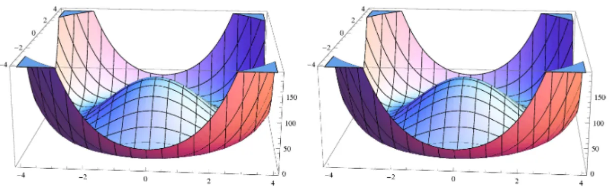
Figure 1: Two wine bottles and the propagation of spin

waves

which

are

orthogonal

or

perpendicular. It costs energy tochangetheradius ofthebottlesbutit iseasy tofluctuate

perpendicular to the radius. This is caused by $\xi$, the massive Gaussian field of $N-1$

degrees offreedom.

Fluctuations $\xi_{n}(x)$ perpendicularto $\phi_{n}(x)$ have $N-1$ degrees of freedom ofGaussian

fields. See also the figure caption. We replace $\varphi_{n+1}\varphi_{n+1}$ by $N\mathcal{G}_{n+1}$ and expand the

determinant up to the second order:

(4.1) $=$ $\int\exp[i\langle\lambda,p\rangle-N\langle\lambda, (\mathcal{T}_{n}^{02}+2\mathcal{G}_{n+1}\circ \mathcal{T}_{n})\lambda\rangle]$ $\cross\det_{3}^{-N/2}(1+2i\Gamma_{n}^{1/2}Q^{+}\mathcal{A}_{n}^{+}\lambda \mathcal{A}_{n}Q\Gamma_{n}^{1/2})$

$\cross\exp[-2\langle\lambda, (:\varphi_{n+1}\varphi_{n+1} :)\circ \mathcal{T}_{n})\lambda\rangle+$ (higher order terms)] $\prod d\lambda(x)$

$\sim \exp[-\frac{1}{4N}\langle p, \frac{1}{2\mathcal{G}_{n+\mathring{1}}\mathcal{T}_{n}+\mathcal{T}_{n^{02}}}p\rangle]$ (4.2)

The terms: $\varphi_{n+1}\varphi_{n+1}$ :

are

treated by polymer expansion and yield relevant terms $\langle$:

$\varphi_{n+1}^{2}$ :,

$g_{n}$ : $\varphi_{n+1}^{2}$ which are fractions of$\log(\varphi_{n}^{2})$.

Putting$p=Ap_{1}+\tilde{Q}\tilde{p}$ with$p_{1}=C^{n+1}p$ and $C^{n+1}A=1$_, _we

_see

_that $P(p)$ is given by

$\exp[-\frac{1}{4N}\langle p_{1},$ $\frac{1}{C^{n}[2\mathcal{G}_{n+1}\circ \mathcal{T}_{n}+\mathcal{T}_{n}^{02}](C^{+})^{n}}p_{1}\rangle_{\Lambda_{n+1}}-\frac{1}{4N}\langle\tilde{Q}\tilde{p},$$\frac{1}{2\mathcal{G}_{n+\mathring{1}}\mathcal{T}_{n}+\mathcal{T}_{n^{02}}}\tilde{Q}\tilde{p}\rangle]$

(4.3)

Here we remind the reader that

$C^{n+1}\mathcal{T}_{n}(C^{+})^{n+1} = 0$

(11)

since $\mathcal{T}_{n}=\mathcal{A}_{n}Q\Gamma_{n}Q^{+}\mathcal{A}_{n}^{+},$ $C^{n}\mathcal{A}_{n}=1,$ $CQ=0$ and $\mathcal{T}_{n}$ decays much

faster than

$\mathcal{G}_{n}$

.

This

means

that the blockwise constant part $p_{1}$ of$p$ remains and the

zero-average

fluctuation

part $\tilde{Q}\tilde{p}$

of$p$ is almost absent since it approximately holds that

$(2\mathcal{G}_{n+1}\circ \mathcal{T}_{n}+\mathcal{T}_{n}^{02})\lceil_{\tilde{Q}\xi}=O(L^{2n})\beta_{n+1}$

though this has to be taken with

a

grain of salt. (We need

a

suble discussion

on

this

point, however.) [step 3]

We

calculate the next order

Gibbs

factor by multiplying the distribution

function

$P(p)=Prob(p=q(\xi))$ to the previous

Gibbs

factor. This idea perhaps goes back to [22]. Inthe presentcase, however, $g_{n}$ canbe large $(\sim L^{2} on A_{n})$ and then we choose$p$which

minimizes

$F(p)$ $=$ $\frac{1}{4N}\langle p,$ $\frac{1}{2\mathcal{G}_{n+\mathring{1}}\mathcal{T}_{n}+\mathcal{T}_{n^{02}}}p\rangle+\frac{1}{4N}\langle(:\varphi_{n+1}^{2}:_{G_{n+1}}+p)$,$g_{n}(:\varphi_{n+1}^{2}:c_{n+1}+p)\rangle$

(4.4)

$= \langle p, \frac{1}{D}p\rangle+\frac{1}{N}\langle(:\varphi_{n+1}^{2}:c_{n+1}, g_{n}p\rangle+\frac{1}{2N}\langle(:\varphi_{n+1}^{2}:_{G_{n+1}g_{n}:\varphi_{n+1}^{2}:c_{n+1}\rangle}$ (4.5)

where

$\frac{1}{D}=\frac{1}{4N}\frac{1}{2\mathcal{G}_{n+\mathring{1}}\mathcal{T}_{n}+\mathcal{T}_{n}^{02}}+\frac{1}{2N}g_{n}$ (4.6)

To diagonalize this,

we

again set$p=\mathcal{A}p_{1}+\tilde{Q}\tilde{p}$ where

$\mathcal{A}=D(C^{+})^{n+1}[C^{n+1}D(C^{+})^{n+1}]^{-1}, C^{n+1}\tilde{Q}=0$ (4.7)

and

$F(p) = F_{1}(p)+F_{2}(p)$ _(4.8a)

$F_{1} = \langle p_{1}, \frac{1}{C^{n+1}D(C^{+})^{n+1}}p_{1}\rangle_{\Lambda_{n+1}}+\frac{1}{N}\langle(:\varphi_{n+1}^{2}:c_{n+1}, g_{n}p\rangle$

$+ \frac{1}{2N}\langle(E:\varphi_{n+1}^{2}:c_{n+1}, g_{n}E:\varphi_{n+1}^{2}:c_{n+1}\rangle$ (4.8b)

$F_{2} = \langle\tilde{Q}\tilde{p}, \frac{1}{D}\tilde{Q}\tilde{p}\rangle+\frac{1}{N}\langle(E^{\perp_{:\varphi_{n+1}^{2}:_{G_{n+1}}}}, g_{n}\tilde{Q}\tilde{p}\rangle$

$+ \frac{1}{2N}\langle(E^{\perp}:\varphi_{n+1}^{2}:c_{n+1}, g_{n}E^{\perp}:\varphi_{n+1}^{2}:c_{n+1}\rangle$ (4.8c)

where $E$ is the projection to block-wise constant functions _{(block of} _size $L^{n+1}\cross L^{n+1}$)

(12)

and $F_{2}$ take their minima at the following points: $p_{1} = - \frac{1}{N}C^{n}Dg_{n}:\varphi_{n+1}^{2}:_{G_{n+1}}$ $= [-1+ \frac{1}{L^{2n}g_{n}}\frac{1}{C^{n}[2\mathcal{G}_{n+1}\circ \mathcal{T}_{n}+\mathcal{T}_{n^{02}}](C^{+})^{n}}]C^{n}:\varphi_{n+1}^{2}:c_{n+1}$ (4.9) $\tilde{Q}\tilde{p}= -\frac{1}{2N}E^{\perp}Dg_{n}:\varphi_{n+1}^{2}:_{G_{n+1}}$ $= [-1+ \frac{1}{9n}\frac{1}{2\mathcal{G}_{n+1}\circ \mathcal{T}_{n}+\mathcal{T}_{n^{02}}}]E^{\perp}:\varphi_{n+1}^{2}:c_{n+1}$ (4.10) Thus

$\min F_{1} = \frac{k}{4N}\langle C^{n+1}:\varphi_{n+1}^{2}:, \frac{1}{C^{n+1}[2\mathcal{G}_{n+1}\circ \mathcal{T}_{n}+\mathcal{T}_{n^{02}}](C^{+})^{n+1}}C^{n+1}:\varphi_{n+1}^{2}:\rangle.$

$\min F_{2}$ $=$ $\frac{1}{4N}\langle E^{\perp}:\varphi_{n+1}^{2}$ :,$\frac{1}{2\mathcal{G}_{n+1}\circ \mathcal{T}_{n}+\mathcal{T}_{n^{02}}}E^{\perp}:\varphi_{n+1}^{2}:\rangle$

We integrate over $p_{1}$ and $\tilde{p}$ around the points (4.9) and (4.10) (steepest descent

method) and we get

some

small terms coming from the integrations over$p_{1}$ and $E^{\perp}\tilde{p}.$

The term $\min F_{1}$

means

that the $9n$ term disappearsand the coeﬃcient oftherelevant

term $(: \varphi_{n+1}^{2}:)^{2}$

can

be regarded

as a

constant for $n>\log\beta$ since $C^{n+1}$ : $\varphi_{n+1}^{2}$ $:\sim:\phi_{n+1}^{2}$ :

(field

on

$A_{n}$) and $C^{n+1}[2\mathcal{G}_{n+1}\circ \mathcal{T}_{n}+\mathcal{T}_{n}^{02}](C^{+})^{n+1}\sim 1$ (on $\Lambda_{n+1}$). This also implies that

$\langle$: $\varphi_{n+1}^{2}:_{G_{n+1}}+p,$$\psi_{n}\rangle$ $arrow$ $\frac{1}{L^{2n}}$$\langle$: $\varphi_{n+1}^{2}:c_{n+1},$$E\psi_{n}\rangle$ (4.11)

which is consistent with

our

choice ofthe scaling of$\psi$ and $\tilde{A}_{n}$

. The term $\min F_{2}$ is

essen-tially $\mathcal{F}_{n}$ which is irrelevant. We remark that the $\log$ term isexpanded and: $\varphi_{n+1}\varphi_{n+1}$ :

is absorbed by $V_{n}^{(1)}$

and the Hamiltonian part of$\phi_{n+1}$ through

$2 :\varphi_{n+1}(x)\varphi_{n+1}(y) \varphi_{n+1}^{2}(x):+:\varphi_{n+1}^{2}(y):-:(\varphi_{n+1}(x)-\varphi_{n+1}(y))^{2}$ :

The shifts ofthe variables $p_{1}$ and

$\tilde{Q}\tilde{p}$

are

in the admissible deviations of $\varphi_{n+1}$ and $q_{n}.$

[step 4]

Thus we can iterate these steps. The most important point is that $q=:\varphi_{n}^{2}$ : –: $\varphi_{n+1}^{2}$ :

obeys theGaussiandistribution uniformly in $n$ (CLT) and the coupling constant $g_{n}$is kept

as a

constant

on the

shell: $\phi_{n}^{2}:_{G_{n}}=0$

near

which the functional integrals have supports.

This ensures our scenario.

5 Remaining

Problems

(13)

1.

Provethis for small $N.$

2. Prove this for quantum spins.

3.

Solvethe Millennium problem of quark confinement.

The present author hopes that the reader is ambitious enough to attack these problems. Acknowledgements. This work

was

partially supported by the

Grant-in-Aid

for

Scientific

Research, No.23540257, No. 26400153, the Ministry of Education,

Science

and Culture,

Japanese

Government.

Part of this work

was

done while the author

was

visiting

INS

Lyon, ${\rm Max}$Planck Inst. for Physics (Muenchen) and UBC (Vancouver.) Hewould like to

thank K.Gawedzki, E.Seiler and D.Brydges for useful discussions and kind hospitalities extended to him. Last but not least, he thanks T. Hara and H.Tamura for stimulating

discussions and encouragements.

References

[1] K. Wilson, Phys. Rev. D10,

2455

(1974) and Rev. Mod.Phys., 55,583 $(1983)_{1}$

A.Polyakov, Phys. Lett 59B,

79

(1975).

[2] D. Brydges,

J.

Dimock and P.Mitter, Note

on

$0(N)\phi^{4}$ models, unpublished paper

(2010, private communication through D.Brydges)

[3] D. Brydges, J. Fr\"ohlich and T. Spencer, Comm. Math. Phys.83 (1982)

123.

[4] D. Brydges, J. Fr\"ohlich and A. Sokal, Comm. Math. Phys. 91 (1985)

117.

[5] D. Brydges, A Short Course

on

Cluster Expansions, in Les Housch Summer School, Session XLIII (1984), ed. by K.Osterwalder et al. (Elsevier

Sci.

Publ., 1986).

[6] S. Caracciolo, R. Edwards, A. Plisetto and A. SokaJ, Phys. Rev. Letters, 74,(1995)

2969:

75, (1996) 1891.

[7] J.

Fr\"ohlich,

R. Israel, E.H. Lieb and B. Simon, Commun.Math.Phys.

62

(1978)

1.

[8] G.Gallavotti, Mem. Accad. Lincei, 14,1 (1978).

[9] K.Gawedzki and A.Kupiainen, Commun. Math. Phys. 99 (1985), 197;

see

also Ann.

Phys., 148 (1983),

243.

(14)

[11] J. Glimm, A. Jaﬀe and T. Spencer, The Particle Structures of the Weakly Coupled

$P(\Phi)_{2}$ Models and Other Applications, Part II : The cluster expansion, in

Construc-tive Quantum Field Theory, Lecture Note in Physics, 25 (1973) 199, ed. by G.Velo

and A. Wightman, (Springer Verlag, Heidelberg, 1973)

[12] K.R.Ito, Phys. Rev. Letters 55(1985) pp.558-561; Commun. Math.Phys. 110 (1987) pp. 46-47; Commun. Math.Phys. 137 (1991) pp.

45-70.

[13] K.R.Ito, Phys. Rev. Letters 58(1987) pp.439-442

[14] K. R. Ito, T. Kugo and H. Tamura, Representation of $0(N)$ _Spin _Models _by

Self-Avoiding Random Walks, Commun. Math. Phys.

183

(1997)

723.

[15] K. R. Ito, and H. Tamura, N dependence of Critical Teperatures of 2D $0(N)$ Spin Models Commun. Math. Phys., (1999), to appear; Lett. Math. Phys. 44 (1998)

339.

[16] K. R. Ito, Renormalization Group Recursion Formulas andFlow of2D $O(3)$ Heisen-berg Spin Models, in preparation (2014, March).

[17] S. K. Ma, The $1/n$ expansion, in Phase Transitions and Critical Phenomena, 6,

249-292, ed. by C. Domb and M. S. Green (Academic Press, London, 1976) [18] M. McBryan and T. Spencer, Commun. Math. Phys. 53, (1977)

299.

[19] V. Rivasseau, From Perturbative to Constructive Renormalization, Princeton Series

in Physics (Princeton Univ. Press, Princeton, N.J., 1991.)

[20] V.Rivasseau, ClusterExpansion with Small/LargeField Conditions, in Mathematical

Quantum Theeory I: Field Theory and Many-Body Theory, ed. by J.Feldman et al., (CRM Proceedings and Lecture Notes, Vol.7, A.M.S., 1994)

[21] E. Seiler, Commun. Math. Phys., 42 (1975)