九州大学応用力学研究所所報
ISSN 1345-5664
No.157
March 2020
CONTENTS
Transient global modeling of oxygen and carbon segregations during the pulling process of
Czochralski silicon crystal growth
By Xin LIU, Hirofumi HARADA, Yoshiji MIYAMURA, Xue-Feng HAN, Satoshi NAKANO,
Shin-ichi NISHIZAWA, and Koichi KAKIMOTO ... 1
3D Numerical Study of Crystal Rotation Effect on Three-Phase Line in Floating Zone Silicon
By Xue-Feng HAN, Xin LIU, Satoshi NAKANO, Hirofumi HARADA, Yoshiji MIYAMURA,
and Koichi KAKIMOTO………...……….….7
Impact of applying tidal correction to marginal-sea bathymetry dataset
Reports of Research Institute for Applied Mechanics, Kyushu University No.157 (1-6) March 2020
Transient global modeling of oxygen and carbon
segregations during the pulling process of Czochralski
silicon crystal growth
Xin LIU
*1, Hirofumi HARADA
*1, Yoshiji MIYAMURA
*1, Xue-Feng HAN
*1,
Satoshi NAKANO
*1, Shin-ichi NISHIZAWA
*1, and Koichi KAKIMOTO
*1 E-mail of the corresponding author: [email protected](Received January 27, 2020)
Abstract
Transient global modeling of the Czochralski silicon (CZ-Si) crystal growth process is essential for understanding the dynamic behaviors of the heat and mass transport in the crystallization set-up. Furthermore, segregation of impurities and dopants could also be predicted dynamically by the transient global simulation. The transient global model for the crystal pulling process was developed for CZ-Si growth with the cusp-shaped magnetic field (CMF). The radial and axial homogeneities of oxygen and carbon were investigated for the growing crystal. The oxygen concentration along the axis decreased with the increase of the length of the crystal. Due to the continuous contamination and the lower segregation coefficient, the carbon concentration increased with the increase of the crystal length. The developed transient global model is also applicable for the segregation prediction of other dopants and impurities in CZ-Si growing process.
Keywords: Computer simulation, Impurities, Mass transfer, Czochralski method
1. Introduction
Large-scale monocrystalline silicon (Si), grown by the Czochralski silicon (CZ-Si) process, has become the most widely used material for power devices, as well as large-scale integrated circuits 1). The quality, purity, and defect-free
nature of these crystals are the prerequisites for their technological applications. To stabilize the crystal growing process, the application of magnetic fields in CZ-Si growth (MCZ-Si) has been established as a standard method to control the melt convection, impurity transport, and growth interface shape 2).
Owing to the low cost and high visualization capability, numerical simulation has become an indispensable tool in the development of efficient time- and cost-saving optimization procedures. CZ-Si growth is a batch-wise process, which means that no steady state can exist. Dynamic effects are very complex due to different time scales, such as melt flow, solid conduction, and crystal pulling. Transient global modeling of the CZ-Si crystal growth process has long been proposed to understand the dynamical behaviors of heat and mass transport in the crystallization set-up 3-7). It is well known that crystal
quality strongly depends on the melt flow, which exerts a
major influence on the melt–crystal (m–c) interface and deeply affects defect formation and oxygen incorporation into the crystal 8). However, most of the transient global simulations
for CZ-Si crystal growth neglected the melt flow and mass transport due to the complexity of convection modeling 3, 4, 9).
It is impossible to reproduce the segregation curves of the impurities and dopants without the predication of coupled melt convection and mass transport. Moreover, MCZ-Si crystal growth with active control of heat and mass transport induces multiple physical phenomena, which is therefore a very challenging task for numerical modeling.
Oxygen (O) is the inevitable impurity in the MCZ-Si growth, which affects the electronic performance and mechanical strength of the Si wafer. The concentration and homogeneity in the grown Si crystal are the key factors for generating O precipitates and O related defects. Furthermore, carbon (C) is an undesirable contamination, which degrades the characteristics of the Si wafers via the formation of C-induced defects. The radial and axial uniformities of O and C in crystals are preferred for CZ-Si crystal growth where the O segregation of O and C accumulation are both the functions of the crystal pulling time. Therefore, the transport and segregation of O and C must be investigated for the entire pulling process. However, most of the transient global simulations for the CZ-Si crystal growth have neglected the
Xin LIU et al.: Transient global modeling of O and C segregations of Czochralski silicon crystal growth
melt flow and mass transport because of the complexity of convection modeling even though reproducing the segregation curves of the impurities and dopants is impossible without the information of the dynamically all-coupled melt convection and mass transport.
The present study develops a transient global model for the crystal pulling process for the CZ-Si growth with a cusp-shaped magnetic field (CMF). The generation, transport, and segregation of O are considered for the crystal growing process. The incorporation, accumulation, and segregation of C are also predicted based on our previous studies on CZ-Si growth 10, 11). Additionally, the CMFs with the varying
zero-Gauss plane (ZGP) locations were investigated and compared. The O and C segregations were plotted as the function of crystal length and radius.
2. Transient global modeling of heat and
mass transport
2.1 Parameters of the transient global simulations
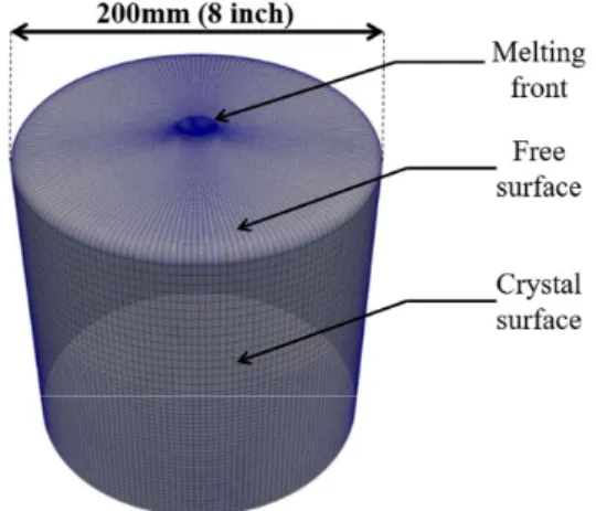
Fig. 1 Configuration and global thermal field of a 300 mm CZ-Si crystal growth with CMF.
The schematic diagram in Fig. 1 shows an industrial Czochralski furnace with the CMF. The diameter and the initial length of the crystal were 306 mm and 50 mm, respectively, and the diameter of the crucible inside wall was 775 mm. The rotation rates of the crucible and the crystal were
4
c rpm
and s 8rpm , respectively; the crystal pulling rate was 0.4 mm/min. The crystal was pulled from a length of 50 mm to 1600 mm at a fixed diameter. The CMFs
with varied ZGP locations were investigated, as presented in Figs. 2(a) to (c). The CMF with its ZGP along the melt free surface was set as the reference case with ZGP = 0. The magnetic field density distribution of CMF is described by
0/ c 2 0
BB R xi yj z H k , whereR and c H are 0
the radius of the crucible and the location of the ZGP, respectively. For different CMF cases, B00.2T was
constant, while ZGP = −100 mm, 0 mm, and +100 mm was imposed in global simulations. The methodology for the transient global simulation of the coupled heat and mass transport and the implementation of the coupled boundary conditions of the CZ-Si crystal growth have been presented in detail in our previous paper 12).
2.2 Impurity (O and C) transport and boundary conditions
The governing equations for O and C transport in the Si feedstock are written as follows:
2 2 Si O O Si i O eff i i c u c D c t x x , (1)
2 2 Si C C Si i C eff i i c c u c D t x x , (2) where c , O c , C Si and u are the molar concentrations iof O and C atoms, the density of Si melt and the velocity vectors, respectively. The turbulent transport of the impurities was considered by introducing the effective diffusivity defined
/ /
eff t t
D Sc Sc . To consider the effect of the turbulent motion in the melt, the Reynolds-averaged Navier–Stokes equation was used with the renormalization group (RNG) k−ε model 13). The molecular and turbulent Schmidt numbers used
were 10 and 0.9, respectively 14). The sharp O concentration
gradient concentration in the boundary layer near the crucible wall and the m–c, and gas/melt interfaces was captured by refining the grids showing the melt in these regions. The material properties used in this study were the same as those used in our previous studies 15).
The following equation, which was obtained from an O solubility measurement performed by Huang et al. 16), was
applied as the boundary condition at the melt–crucible interface:
19 3 1.32 10 exp 3.20 10 / O c T (atoms cm ), (3)3where T is the melt temperature. The O evaporation at the melt free surface was considered according to the
measurements of Togawa et al. 17) given as follows:
/ ( )
eff O O
D c n T c
, (4) where the evaporation rate coefficient
7 4
( ) 5.9152 10 exp 4.1559 10 /T T
. (5) The following boundary condition of the O concentration at the m–c interface is given when the segregation coefficient of
Xin LIU et al.: Transient global modeling of O and C segregations of Czochralski silicon crystal growth
3 O at the growth interface is assumed to be unity:
/ 0
O
c n
. (6) A zero-flux boundary condition was used for C on the crucible wall. The C contamination flux at the melt free surface was considered according to our previous study 11).
Further, based on the results of the melting process modeling and validations, we set the final C and contamination flux obtained as the initial and boundary conditions of the melt free surface for the pulling process modeling. The segregation coefficient (k ) of C at the m–c interface was assumed to be seg 0.07. The boundary condition of C concentration at the m–c interface is given as follows:
1
0 C eff g C seg c D V c k n , (7) where V is the crystal pulling rate. g(a)
(b)
(c)
Fig. 2 Schematic of the investigated CMF configurations with different ZGPs: (a) ZGP = −100 mm; (b) ZGP = 0; and (c) ZGP = +100 mm.
3. Results and discussion
Transient global simulations were performed for the pulling process of the MCZ-Si crystal growth. The thermal field, melt flow, and impurity transport under the effect of the CMF were predicted with coupled boundary conditions of heat, flow, and mass transport. The generation, transportation, and segregation of O and C in the Si domain were also considered for the diameter growth stage. Three cases with different CMF configurations were considered to clarify the mechanisms of the impurity uniformities in the radial and axial directions.
3.1 Effects of the CMF on O transport and segregation
(a)
(b)
(c)
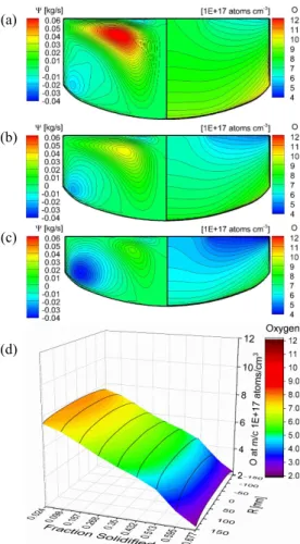
(d)
Fig. 3 Melt flow and O transport for the reference case with ZGP = 0 in the CMF. (a) Stream function and O contours for the solidified fraction (f ) = 0.15; (b) stream function and O s contours for the solidified fraction (f ) = 0.30; (c) stream s
function and O contours for the solidified fraction (f ) = 0.45; s and (d) distribution of O at the m–c interface during the pulling process.
Figs. 3(a) to (c) present the stream function and O contours, respectively, for the reference case with the CMF of ZGP = 0 for different solidified fractions. The positive and negative values of the stream function denote the
Xin LIU et al.: Transient global modeling of O and C segregations of Czochralski silicon crystal growth
anticlockwise and clockwise flow patterns, respectively. The melt had three clear vortices, as shown in the left sections of Figs. 3(a) to (c). Despite cases where the flow structures were similar for different solidified fractions, the strengths of the melt flow varied with the decrease in the Si melt amount. The clockwise vortex near the corner of crucible wall is the buoyant flow. The clockwise under the m-c interface is the crystal rotation effect. The flow cell between the buoyant and crystal rotation cells shrunk with the crystal pulling process, which was favorable for the reduction of O segregated from the m-c interface. This vortex could take the O from the bottom wall of the crucible to the crystallization zone under the m-c interface.
The O dissolved from the crucible wall was transported to the melt free surface and m–c interface. Different O concentration levels and radial uniformities were observed at the m–c interface. The O distribution in the core region was dominated by the turbulent transport, which was modeled by the eddy viscosity. With the increase in the solidified fraction ( f ) from 0.15 to 0.45, the dissolution area decreased along s with the maximum temperature of the crucible wall. These combined effects led to the inhomogeneous O contents in the crystal along the pulling axis, as shown in Fig. 3 (d). The crystal rotation effect could ensure the radial uniformity of O at the m–c interface from the initial to the final stage of pulling.
3.2 O transport and segregation for different ZGP locations in the CMF
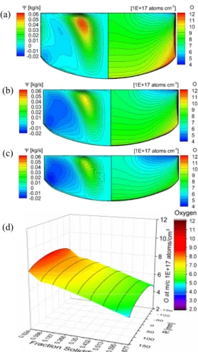
Figs. 4(a) to (c) present the stream function and O contours, respectively, for the case with ZGP = −100 mm in the CMF for different solidified fractions. A significant variation in the flow structure in the melt was observed for different solidified fractions. The entire melt was exposed to a lower magnetic field intensity compared to the reference CMF case of ZGP = 0 because the ZGP was located in the melt domain. The flow structures of the case with ZGP = −100 mm significantly varied in the melt for different solidified fractions. The buoyant cell gradually dominated with the increasing solidified fraction, which was favorable for the reduction of O incorporation. The contours of O in the right section of Figs. 4(a) to (c) exhibit a strong correlation with the depth of the melt in the crucible and the flow structure inside the melt. The O level at the m–c interface experienced a rapid decrease followed by a final increase in its level, as shown in Fig. 4(d). This tendency was similar to the experimental measurement of the O segregation curve in a conventional CZ-Si growth [14]. However, the rapid decrease or increase of O is detrimental to the axial uniformity of O in the crystal.
Figs. 5(a) to (c) illustrate the stream function and O contours, respectively, for the case with ZGP = + 100 mm in the CMF for different solidified fractions. The flow structures
in the melt were very stable for the different solidified fractions. The whole melt was exposed to a higher magnetic field intensity compared to the reference CMF case of ZGP = 0 because the ZGP was located in the crystal domain. The Lorentz force was sufficiently strong to stabilize the melt convection. However, the vortex under the melt free surface could transport the melt with rich O to the m–c interface. The O levels at the m–c interface were higher than the corresponding solidified fractions in the reference CMF cases, as shown in the right sections of Figs. 5(a) to (c). The O level at the m–c interface experienced a gradual decrease during the entire pulling process, as shown in Fig. 5 (d). However, its radial uniformity was poor because of the weakened crystal rotation effect, which was suppressed by the Lorentz force.
(a)
(b)
(c)
(d)
Fig. 4 Melt flow and O transport for the reference case with ZGP = − 100 mm in the CMF. (a) Stream function and O contours for the solidified fraction ( f ) = 0.15; (b) stream s
function and O contours for the solidified fraction (f ) = 0.30; s
(c) stream function and O contours for the solidified fraction ( f ) = 0.45; and (d) distribution of O at the m–c interface s
during the pulling process.
In summary, the comparison of the O transport and segregation for the different ZGP locations revealed that the O level and uniformities at the m–c interface were strongly
Xin LIU et al.: Transient global modeling of O and C segregations of Czochralski silicon crystal growth
5 correlated with the depth of the melt in the crucible and the flow structures inside the melt. In the lower ZGP, the lowest O concentration was observed despite the worst axial uniformity, which was due to residual buoyancy convection as shown in Fig. 6. The middle ZGP could maintain the crystal rotation effect and obtain the best radial uniformity of the O concentration at the m–c interface. The higher ZGP significantly stabilized the melt convection; hence, the O segregation curve was flattened, but with higher O level and worse radial uniformity. These comparisons indicated that the adjustments of the ZGP in the CMF have the potential to optimize the O segregation into the pulling crystal from the level, axial, and radial uniformities.
(a)
(b)
(c)
(d)
Fig. 5 Melt flow and O transport for the reference case with ZGP = + 100 mm in the CMF. (a) Stream function and O contours for the solidified fraction ( f ) = 0.15; (b) stream s
function and O contours for the solidified fraction (f ) = 0.30; s (c) stream function and O contours for the solidified fraction ( f ) = 0.45; and (d) distribution of O at the m–c interface s during the pulling process.
3.3 C transport and segregation for different ZGP locations in the CMF
The effects of the different ZGP locations in the CMF on
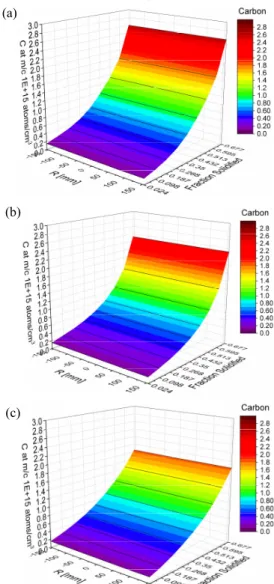
C transport and segregation were also investigated using the transient global simulations. Figs. 7(a) to (c) show the C concentrations at the m–c interface for the different ZGP locations in the CMF. The C accumulation in the melt during the pulling process resulted in the continuous increase in the C concentration at the m–c interface. The radial distributions of C were very homogenous because of the mixing effect of the melt convection. Despite similar contamination flux from the melt free surface, the C incorporation rate into the pulling crystal was different for different ZGP locations in the CMF. The CMF of ZGP = −100 mm showed the highest C contamination rate, while that of ZGP = +100 mm presented a minimum C contamination rate. It indicates that the Lorentz force with higher intensity retarded the melt flow and the C segregation into the pulling crystal.
Fig. 6 Segregation curves of O as the function of the crystal pulling length for the CMF configurations with different ZGPs.
4. Conclusion
In this study, we conducted a series of transient global simulations for the pulling process with different ZGPs in the CMF to elucidate the transport and segregation of O and C in the MCZ-Si crystal growth. The O and C distributions at the growth interface were dynamically predicted for the pulling stages. The O and C segregations were plotted as a function of the crystal length and solidified fraction. The O level and uniformities at the m–c interface were strongly correlated with the depth of the melt in the crucible and the flow structures inside the melt. In the lower ZGP, the lowest O concentration was observed despite the worst axial uniformity. The middle ZGP maintained the crystal rotation effect and obtained the best radial uniformity of O concentration at the m–c interface. Because the upper ZGP stabilized the melt convection significantly, the O segregation curve was flattened, but with higher O level and worse radial uniformity. The intensive Lorentz force retarded the melt flow and the C segregation into the pulling crystal. The adjustments of the ZGP in the CMF
Xin LIU et al.: Transient global modeling of O and C segregations of Czochralski silicon crystal growth
have the potential to optimize the O and C segregations into the pulling crystal from the level, axial, and radial uniformities. Additionally, the developed dynamic global model has applications in the segregation prediction of other dopants and impurities in the CZ-Si growing process.
(a)
(b)
(c)
Fig. 7 C distributions at the m–c interface during the pulling process for the CMF configurations with different ZGPs: (a) ZGP = −100 mm; (b) ZGP = 0; and (c) ZGP = +100 mm.
Acknowledgment
This work was partially supported by the New Energy and Industrial Technology Development Organization (NEDO) under the Ministry of Economy, Trade and Industry (METI), Japan.
References
1) G. Eranna, Crystal Growth and Evaluation of Silicon for VLSI and ULSI, CRC Press, New Youk (2014).
2) J. J. Derby and R. A. Brown, Journal of Crystal Growth, 83,
137 (1987).
3) V. M. Mamedov, M. G. Vasiliev and V. S. Yuferev, Journal of Crystal Growth, 318, 703 (2011).
4) A. Sabanskis, K. Bergfelds, A. Muiznieks, T. Schröck and A. Krauze, Journal of Crystal Growth, 377, 9 (2013). 5) P. D. Thomas, J. J. Derby, L. J. Atherton, R. A. Brown and M. J. Wargo, Journal of Crystal Growth, 96, 135 (1989). 6) N. Van den Bogaert and F. Dupret, Journal of Crystal Growth, 171, 65 (1997).
7) N. Van den Bogaert and F. Dupret, Journal of Crystal Growth, 171, 77 (1997).
8) K. Hoshikawa and X. Huang, Materials Science and Engineering: B, 72, 73 (2000).
9) G. Müller, A. Mühe, R. Backofen, E. Tomzig and W. v. Ammon, Microelectronic Engineering, 45, 135 (1999). 10) X. Liu, B. Gao and K. Kakimoto, Journal of Crystal Growth, 417, 58 (2015).
11) X. Liu, H. Harada, Y. Miyamura, X.-f. Han, S. Nakano, S.-i. Nishizawa and K. Kakimoto, Journal of Crystal Growth, 499, 8 (2018).
12) X. Liu, H. Harada, Y. Miyamura, X.-f. Han, S. Nakano, S.-i. Nishizawa and K. Kakimoto, Journal of Crystal Growth, 532, 125405 (2020).
13) T. Zhang, G. X. Wang, H. Zhang, F. Ladeinde and V. Prasad, Journal of Crystal Growth, 198-199, 141 (1999). 14) A. D. Smirnov and V. V. Kalaev, Journal of Crystal Growth, 310, 2970 (2008).
15) X. Liu, L. Liu, Z. Li and Y. Wang, Journal of Crystal Growth, 354, 101 (2012).
16) X. Huang, K. Terashima, H. Sasaki, E. Tokizaki and S. Kimura, Japanese Journal of Applied Physics, 32, 3671 (1993).
17) S. Togawa, X. Huang, K. Izunome, K. Terashima and S. Kimura, Journal of Crystal Growth, 148, 70 (1995).
Reports of Research Institute for Applied Mechanics, Kyushu University No.157 (7 – 11) March 2020
3D Numerical Study of Crystal Rotation Effect on
Three-Phase Line in Floating Zone Silicon
Xue-Feng HAN
*1, Xin LIU
*1, Satoshi NAKANO
*1,
Hirofumi HARADA
*1, Yoshiji MIYAMURA
*1and Koichi KAKIMOTO
*1 E-mail of corresponding author: [email protected](Received January 28, 2020)
Abstract
In this paper, we have developed a model for a 200 mm floating zone silicon crystal growth process to investigate solid–liquid interface. To study the effect of high-frequency (HF) electromagnetic (EM) heating on the solid-liquid interface shape, HF-EM and heat transfer calculations were conducted in three dimensions. By considering 3D Marangoni and EM forces at the free surface, a more accurate interface shape has been obtained. the results showed that local growth rate became more inhomogeneous when the rotation speed of the crystal was increased. However, a more homogeneous three-phase line could be obtained with a high rotational crystal speed.
Keywords: Computer simulation, Floating zone technique, Semiconducting silicon
1. Introduction
Floating zone (FZ) silicon is used in high-voltage power devices with its low impurity levels [1]. One of the challenges in competing with Czochralski (CZ) silicon lies in increasing the diameter of the crystal. For CZ silicon, crystals with a 300 mm diameter are already being produced commercially and studied [2]. The limitations of increasing the diameter of FZ silicon crystal are mainly because relatively high electrical power increases the possibility of arcing in the region of the electromagnetic (EM) current supplies [3]. The solidification front easily breaks out in the radial direction. To solve the arcing problem, H. J. Rost et al. [4] suggested using low frequency (1.7 MHz) to grow FZ crystals. For the breaking out problem, it is believed that deflection of the three-phase line causes melt spillage. R. Menzel calculated the current density along the three-phase line, indicating that the current density becomes more inhomogeneous with increasing crystal diameter [5]. High power density below the current supplies causes deflection of the three-phase line and the breaking out problem.
To analyze the complex flow and three-dimensional phenomena, a three-dimensional numerical model is
required. There are numerous previous studies on the simulation of 100 mm FZ silicon crystal growth [6-10]. A. Sabanskis et al. [6] have modeled the doping process from the gas in FZ process and compared the calculation result with the experimental data. The influence of cooling gas also has been discussed through axis-symmetric global simulation [7]. G. Ratnieks et al. calculated phase boundaries, temperature distribution, and dopant concentration for 100 mm FZ silicon [8, 10, 11]. The melt flow caused by EM force and Marangoni force have been discussed in three dimensions. G. Ratnieks [11] also proposed a 2D axis-symmetric simulation model of 200 mm FZ silicon to investigate the phase boundary and compare it with experimental result.
However, there has been no reported numerical study of three-dimensional 200 mm FZ silicon to investigate the deflection of the three-phase line. The deflection could hinder further increases in FZ silicon crystal diameter. Therefore, in the present study, we proposed a three-dimensional 200 mm FZ model to analyze the deflection of the three-phase line.
2. Numerical models
Fig. 1 shows the EM model for calculation of the EM field in the FZ process. The dimensions of the feed rod, crystal, and inductor coil are referred to in previous
*1 Research Institute for Applied Mechanics, Kyushu Univ.
Han et al.: 3D Numerical Study of Crystal Rotation Effect on Three-Phase Line in Floating Zone Silicon
research [11]. The diameter of the feed rod is 150 mm. The diameter of the crystal is 200 mm. There are three side slits and one main slit in the induction coil. The induction heating is operated at a high frequency of around 3 MHz. Induction heating and EM force are neglected in the domain deeper than skin depth. Skin depth is 0.26 mm in the silicon melt when the working frequency is 3 MHz. Compared to the calculation domain of silicon of several hundred millimeters, the skin depth is considered the boundary of the calculation domain. The impedance boundary condition is used to model the skin depth effect.
The simulation domain is the space between the crystal and the furnace. The boundary of the model is the
surface of the crystal, melt and inductor. The magnetic and electric fields are expressed in terms of the magnetic vector potential 𝑨 and the electric scalar potential 𝑉. The governing equation to solve the time-harmonic equation can be written as:
𝜵 × (𝜇 𝜵 × 𝑨) + 𝜎𝜵𝑉 + 𝑗𝜔𝜎𝑨 = 𝑱𝒆 (1) where σ is electrical conductivity, 𝜇 is the permeability, 𝑗 is an imaginary unit, 𝜔 is the angular frequency, and 𝑱𝒆
is the externally generated current density. The calculation for 3D EM field is conducted by the AC/DC simulation module in the commercial software COMSOL.
Heat transfer and fluid flow calculations are conducted using open-source library OpenFOAM 2.3.1. Fig. 2 shows the calculation model for heat transfer and fluid flow. The phase boundary of silicon is assumed to be fixed. The free surface of the melt and melting front are obtained from the previous study of 200 mm FZ silicon [11]. The free surface and melting front are assumed to be axis-symmetric.
The crystallization interface is calculated. The shape of the crystallization interface is coupled with the
temperature field. The rotation of the crystal is considered. The heat transfer calculation was conducted using the finite volume method. The governing equations in the steady-state melt flow are the continuity equation (Eq. (2)) and the Navier–Stokes equation (Eq. (3)):
𝜵 ∙ (𝜌𝑼) = 0 (2)
𝜵 ∙ (𝜌𝑼𝑼) = 𝜵 ∙ (𝜇𝜵𝑼) − 𝜵𝑝 + 𝜌𝑔 (3) where 𝜌 is the melt density, 𝑼 is the velocity vector in the melt, 𝜇 is the viscosity of the melt, p is the pressure, and 𝑔 is the gravitational acceleration constant. The heat transfer in the melt and crystal is solved by the following equation:
𝜌𝑼𝜵ℎ = 𝜵 ∙ (𝑎𝜵ℎ) (4)
where ℎ is enthalpy and 𝑎 is thermal diffusivity.
3. Results
During the FZ process, direct heating from the induction coil leads to a high temperature at the free surface of the silicon melt. This technique causes a high gradient of temperature and electromagnetic flux density. The Marangoni and EM forces at the free surface contribute to melt flow at the free surface, which was reported in the previous study [12]. Fig. 3a shows the calculated current density distribution at the free surface. Below the tips of the three side slits, the current density is higher. Below the main slit, the current density is lower. In the vicinity of the current supplies, the current density is higher.
By using the current density distribution at the free surface, the heating power at the free surface was calculated. Accordingly, the temperature and flow field
Fig.1 3D numerical model for high-frequency EM field in the FZ growth system.
Fig.2 3D model for heat transfer calculation. The melt and crystal are included in the same calculation domain. The diameter of the crystal is 200 mm. The model consists of structured mesh.
Han et al.: 3D Numerical Study of Crystal Rotation Effect on Three-Phase Line in Floating Zone Silicon
9 were calculated. Fig. 3b shows the temperature distribution at the free surface. Below the tip of the side slits, the temperature is high because of the high power density. Below the main slit, the temperature is low because of the low power density. The temperature field is not symmetric, which is affected by the flow and the rotation of crystal. The maximum temperature difference is 70 K in the melt. The temperature difference is higher than previous 2D calculation [10] because the maximum temperature of the 2D model is an averaged value along the azimuthal direction.
The shape of the crystallization interface is crucial in FZ silicon crystal growth. Particularly, the periphery of the interface (three-phase line between gas, crystal, and melt) should be stable during growth. Deflection of the three-phase line leads to a lateral growth of crystal.
In Fig. 4, the local growth rate fluctuation is
calculated at the interface under different rotational crystal speeds. The local growth rate fluctuation depends on the rotation speeds of the crystal and azimuthal interface deflection. The pulling rate is the same at
Fig.3 a. Surface current density distribution at the free surface of the melt. b. Temperature distribution at the free surface of melt.
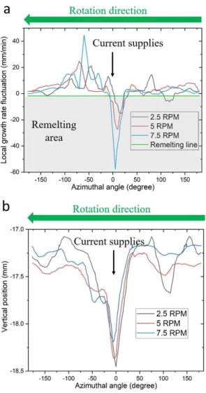
Fig.4 Local growth rate fluctuation at the crystallization interface under crystal rotational speeds of 2.5 RPM, 5 RPM, and 7.5 RPM.
Han et al.: 3D Numerical Study of Crystal Rotation Effect on Three-Phase Line in Floating Zone Silicon
different rotational speeds of the crystal. Different rotational speeds affect the shape of the interface. The variation in local growth rate occurs at the periphery of the interface because of the inhomogeneous EM heating at the three-phase line. Particularly, in the vicinity of the current supplies, a significant negative growth rate occurs. The negative growth rate means that the crystal could melt locally and instantly. When the rotational speed of the crystal is increased, the interface becomes more homogeneous. And the variation in the local growth rate becomes larger.
Fig. 5a shows the local growth rate fluctuation at the three-phase line along the azimuthal direction. Below the current supplies, the local growth rate fluctuation is negative in different crystal rotational speeds. In the
cases of 2.5 RPM, 5 RPM, and 7.5 RPM, the minimum local growth rate fluctuations were approximately −18 mm/min, −28 mm/min, and −57 mm/min, respectively. This means that the temporal re-melting phenomenon is more significant at high crystal rotational speeds. Moreover, the maximum local growth rate fluctuation also increased when the rotational speed of the crystal increased.
Fig. 5b shows the vertical positions of the three-phase lines at different crystal rotational speeds. The deviation of the vertical position of the three-phase line is < 1.5 mm. In the case of 2.5 RPM, the three-phase line has the lowest position below the current supplies because of strong EM heating under the current supplies. The position of the three-phase line is not homogeneous because EM heating is not homogeneous at the three-phase line. When the speed of the crystal is increased to 5 RPM, the lowest position becomes higher and the three-phase line becomes more homogeneous. The deviation of the vertical position of the three-phase line is decreased to 1 mm when the rotational speed of the crystal is increased to 7.5 RPM. Though the re-melting phenomenon becomes more significant when the rotational speed of the crystal is increased, the duration of the temporal re-melting region is shorter. Therefore, a high rotational crystal speed could improve the homogeneity of the three-phase line.
4. Conclusion
In this paper, a high-frequency EM model and heat transfer model for a 200 mm FZ process are constructed. The FZ model presented in the paper considered the three-dimensional Marangoni force, EM force, and interface deflection. The local growth rate is also taken into account according to the deflection of interface and rotation speeds. The deflection of the three-phase line is obtained at different rotational speeds of the crystal. The deflection below the current supplies was found to be most significant. The downward deflection has the potential risk of melt spillage from the crystal or lateral growth to break the symmetry of the crystal. At higher crystal rotational speeds, the local growth rate increases in fluctuation. However, the duration of the fluctuating local growth rate is shorter at higher crystal rotational speeds. Therefore, at higher crystal rotational speeds, the three-phase line is more homogenous, and the risk of melt spillage or lateral growth is reduced.
Acknowledgment
This work was partly supported by the New Energy
Fig.5 a. Comparison of the local growth rate fluctuation along the three-phase line among different crystal rotational speeds. The temporal re-melting area is indicated in the shade. b. Comparison of the positions of the three-phase line among different crystal rotational speeds.
Han et al.: 3D Numerical Study of Crystal Rotation Effect on Three-Phase Line in Floating Zone Silicon
11 and Industrial Technology Development Organization (NEDO) under Ministry of Economy, Trade and Industry.
References
1) W. Zulehner, Historical overview of silicon crystal pulling development, Materials Science and Engineering: B, 73,7-15, 2000
2) R. Yokoyama, T. Nakamura, W. Sugimura, T. Ono, T. Fujiwara, K. Kakimoto, Time-dependent behavior of melt flow in the industrial scale silicon Czochralski growth with a transverse magnetic field, Journal of Crystal Growth, 519, 77-83, 2019 3) L. Altmannshofer, M. Grundner, J. Virbulis, Silicon
single crystal produced by crucible-free float zone pulling, in, US Patents, 2005.
4) H.J. Rost, R. Menzel, A. Luedge, H. Riemann, Float-Zone silicon crystal growth at reduced RF frequencies, Journal of Crystal Growth, 360, 43-46, 2012
5) R. Menzel, Growth Conditions for Large Diameter FZ Si Single Crystals, PhD thesis, 2013
6) Sabanskis, K. Surovovs, J. Virbulis, 3D modeling of doping from the atmosphere in floating zone silicon crystal growth, Journal of Crystal Growth, 457, 65-71, 2017
7) Sabanskis, J. Virbulis, Simulation of the influence of gas flow on melt convection and phase boundaries in FZ silicon single crystal growth, Journal of Crystal Growth, 417, 51-57, 2015
8) G. Ratnieks, A. Muiznieks, L. Buligins, G. Raming, A. Mühlbauer, A. Lüdge, H. Riemann, Influence of the three dimensionality of the HF electromagnetic field on resistivity variations in Si single crystals during FZ growth, Journal of crystal growth, 216, 204-219, 2000
9) Mühlbauer, A. Muiznieks, J. Virbulis, A. Lüdge, H. Riemann, Interface shape, heat transfer and fluid flow in the floating zone growth of large silicon crystals with the needle-eye technique, Journal of crystal growth, 151, 66-79, 1995
10) G. Ratnieks, A. Muižnieks, A. Mühlbauer, G. Raming, Numerical 3D study of FZ growth: dependence on growth parameters and melt instability, Journal of crystal growth, 230, 48-56, 2001
11) G. Ratnieks, Modelling of the Floating Zone Growth of Silicon Single Crystals with Diameter up to 8 Inch, PhD thesis, 2007
12) G. Raming, A. Muižnieks, A. Mühlbauer, Numerical investigation of the influence of EM-fields on fluid motion and resistivity distribution during floating-zone growth of large silicon single crystals, Journal of crystal growth, 230, 108-117, 2001
九州大学応用力学研究所所報 第 157 号 (12-26) 2020 年3月
縁辺海海底地形データに対する潮高補正の適用
上原 克人
*1(2020 年 1 月 31 日受理)
Impact of applying tidal correction to marginal-sea bathymetry dataset
Katsuto UEHARA
E-mail of corresponding author: [email protected]
Abstract
A method to convert the reference level of chart depths from the lowest tide level to the mean sea level was developed to improve the quality of bathymetry datasets of the East and South China seas. The conversion was made by referring to a newly compiled database of the offset value (Z0) derived from that listed in tide tables. Numerical
simulations using the revised East China Sea bathymetry revealed that the depth correction lead to 40% reduction of the RMS difference between the predicted and observed M2 tidal amplitudes, mainly due to the changes at regions
with shallow depths and large tidal range such as the Korean west coast and the Southwestern Yellow Sea. It was also found that the global bathymetry dataset GEBCO2019 uses chart depths without applying the correction and the mismatch between the zero level for the land and sea seems to have caused erroneous depths at intertidal zones. Key words: Bottom topography, tidal model, East China Sea, South China Sea
1.
はじめに
潮汐モデルの精度を左右する主要な要素に海底地形が ある。例えば、東シナ海と北西ヨーロッパ陸棚を対象にほぼ 同じ設定で行った2つの潮汐シミュレーションの結果[1-2]を比 較すると、モデル推計値と観測値との間の二乗平均偏差が 前者では M2潮振幅で 17cm、位相で 15 度であったのに対 し、後者はそれぞれ 5.6cm、6.5 度と半分以下であった。似 通った潮汐振動特性を持つ両海域においてモデル間の精 度の差がここまで開いた要因の一つとして、計算に使用した モデル地形の精度の違いが考えられる。このように、潮汐シ ミュレーションの精度向上には海底地形データの信頼性が 重要な意味を持つ。 近年は空間分解能の高い全球地形データセットが公開 され[3-5]、最新の GEBCO2019[5]では世界各地の水深が緯 度・経度ともに 0.25 分(1/240 度、赤道で約 460m)間隔で提 供されている。しかし解像度の向上に品質が伴っているとは 必ずしも言えない。外洋については 1990 年代から利用可能 となった衛星海面高度計データの採用により水深の精度が 飛躍的に向上したが、高度計データの適用が難しい沿岸域 に関しては、測深データの不足や検証の不十分さなどから 非現実的な水深値や海底地形を示す場所が少なくない。 そのため、筆者はアジア縁辺海潮汐モデルの精度向上 を目的とした独自の海底地形グリッドデータを、東シナ海と 南シナ海を対象に構築してきたが[6-9](Fig.1)、作成した地形 データを使って潮汐モデルを駆動したところ、計算値と観測 値との差がむしろ増加してしまった。検証の結果、地形デー タ作成時に使用した海図由来の水深値の取り扱いに問題 があり、岸近くの水深を過小評価していたことがその原因の 一つとして浮上した。 海図水深のゼロ点は低潮時の水面高度(最低水面)に準 拠しており、平均水面から測定した水深とは同じではないが、 従来のデータ作成時にはその差を考慮してこなかった。最 低水面と平均水面の差はたかだか数メートルであり、沖合で は問題にならないが、岸近くの浅海域では無視できない可 能性がある。 本稿は海図水深を平均水面準拠の水深に変換する簡便 な手法を開発し、変換後の水深を用いた海底地形データを 作成するとともに、修正の効果について潮汐モデルを駆動 することにより検証したものである。さらに既存の全球地形デ ータにおいても、近年では浅海域の地形情報を電子海図 収録の水深で積極的に補う傾向が見られることから、同様 の問題が生じていないか、確認を行った。 *1 九州大学応用力学研究所上原 : 縁辺海海底地形データに対する潮高補正の適用 13
2. 海図水深
最初に海図に記載されている水深の定義と、本稿にて行 う水深変換の概要を述べる。海図は航海目的で発行されて いることから、陸上 の地 形図が基準としている平均水 面(MSL=Mean Sea Level)からではなく、座礁の危険性が高まる 低潮時の最低水面(Chart datum)から測った深さを水深とし
て採用している。この海図水深 HCと一般的な水深の定義で
ある平均水面から測った水深 HMは同一視されることが多い
が、Fig. 2 に示すような違いがある。
上原 : 縁辺海海底地形データに対する潮高補正の適用 本稿で扱う「平均水面」と「最低水面」は、観測結果に基 づいているものの、あくまで海図編集時に使用される観念的 な量である。測地学的な厳密さは必ずしも持たない。ここで は、どちらの海面高度も場所ごとに変化するが、時間的には 不変であると仮定する。 これら平均水面ならびに最低水面に準拠した水深は HM = HC + Z0 (1) の関係にある。ここで Z0は平均水面と最低水面との差であり、 慣習的に正値で表される。最低水面は、それ以上下がるこ とが少ない海面高度であり、具体的な定義は国によって異 なる。日本では略最低低潮面(平均水面から潮汐の主要4 分潮の振幅の和だけ低い高度)として定められ[11]、国内各 地の潮位観測に基づく Z0の値が海上保安庁のホームペー ジにて公示されている[12]。Z 0については、験潮所における 値が潮汐表や海図にも記載されている。 さらに、水深測量時の海面から計測した測得水深 Hobsと 海図水深 HCとの間には以下の関係がある。 Hobs = HC + ( Z0 + HT' ) = HC + HT (2) ここで、HT’は測量時の平均水面上の潮位であり、HT’に前 述の Z0を加えた量、すなわち最低水面を基準とした水面の 高さを潮高 HTと呼ぶ。測得水深を海図水深に変換する作 業を潮高補正と呼び、水深測量に際して原則として水深 200m 以浅の場所ではこの補正を行うこととされている。本稿 では、この潮高補正適用後の海図水深を扱い、測得水深は 使用しないことから、以下では HT’を考えず、(1)式に基づく HMと HCの間の変換を潮高補正と呼ぶことにする。 海図において最低水面を基準とした水深を記載するのは 世界共通の手法で、古くから行われている[13]。例えば、 Fig.3a は 1924 年刊行の海図第 60 号「品川湾」の一部を示 したものである。今日の晴海地区や豊洲地区にあたる隅田 川河口の広い範囲に描かれた網掛けは、最低水面より上に 位置する潮間帯を表している。海図では下向きを正にとるこ とから、最低水面より高い場所にあるこれらの海域の水深は 負値(下線付きの数字)として記されている。このような記法 は、今日の海図でも使われている。 浅瀬では、基準面に最低水面と平均水面のどちらにとる かで、見かけの水深が大きく変わる。例えば Fig.3a の隅田 川河口の潮間帯の水深は-0.3m~-0.1m と記されているが、 これは最低水面から測った値である。この海図では海域の 平均水面の高さを最低水面上 1.1m と規定していることから、 平均水面下の水深で表すと 0.8~1.0m と符号が反転する。 同様に Fig.3a 中央下側の澪筋(白く表示された深い溝)の 水深は 0.2m~0.6m と記載されているが、平均水面準拠水 深(HM)に換算すると 1.3m~1.7m である。水深の定義によっ て値が 2~6 倍変わってしまうことになる。 海図水深と平均水面準拠水深の差 Z0は、潮差が大きい 場所では特に顕著となる。大潮差で知られる韓国の仁川港 では Z0が 4.6m、潮間帯の幅は 10km 以上に及ぶ(Fig.3b)。 (a) (b)
Fig.3. Examples of navigational charts showing intertidal zones with shadings. (a) Tokyo Port (Japanese Chart #60 issued in 1924. Courtesy of Institute of Geography, Tohoku University) and (b) Incheon Port, Korean west coast (Japanese chart #326 issued in 1986).
Fig.2. Relation between depths actually measured (Hobs),
depths that refer to chart datum (HM) as indicated in
navigational charts, and those refer to mean sea level (HM). Z0 denotes offset between the two reference levels,
HT "height of tide" shown in tide tables and HT' an
上原 : 縁辺海海底地形データに対する潮高補正の適用 15 数値モデルでは、暗黙のうちに水位のゼロ点を平均水面 と仮定し、水深 0m の位置を海陸境界と仮定していることが 多い。従って浅い沿岸域では潮高補正の有無が計算結果 に大きく影響している可能性がある。 これまで示してきた平均水面や最低水面などの算出は一 定期間の水位観測が必要であり、実際に水深測量が行わ れる沖合では正確な値が得られないことが一般的である。 そのため補正量 Z0の決定には、測量従事者の判断に伴う 任意性が介在する。近年では潮汐モデル結果を活用して 沖合の Z0を推定する試みも進められているが[14, 15]、現状で は測深点近くの験潮所の Z0を援用することが多い。この前 提に立ち、海図水深を平均水面準拠水深に変換する新た な手法を次節以降で示す。
3. 手法
地形データの作成手順を Fig.4 に示す。最低水面に準拠 する一部の水深データを、平均水面準拠の水深に変換す る過程が加わるとともに、変換に必要な Z0に関するデータベ ースを用意する点が従来の版とは異なる。以下では今回の 変更点の詳細並びに検証に用いた潮汐モデルについて説 明する。水深データの取得法など、旧版から変更がない事 項については、前回の報告[9]を参照されたい。 3.1 Z0データベースの作成 平均水面と最低水面の差である Z0の算定には一定期間 の潮位観測が必要であり、験潮所以外ではごく限られた地 点でしか値が得られていない。そのため、ある場所での水深 を変換するには、何らかの手段でその場所の Z0を推定する 必要がある。 略最低低潮面を最低水面として用いる場合、Z0はその場 所の主要4分潮の振幅和に相当する。このことから当初は 数値モデルによって見積もられた主要4分潮の振幅の和を Z0として使うことを検討したが、縁辺海スケールの数値モデ ルでは潮間帯を横切る澪筋を解像できないこともあり、潮間 帯近くの験潮所での Z0の推計値が、観測から得られた値よ り小さめに出てしまうことがわかった。さらに現時点の海図に 記載されている水深の大部分は数値モデルが普及する前 の時代に測深・潮高補正がなされたものであり、モデルで推 定した Z0との親和性が低い可能性が高い。 これらの背景から、本稿では水深測量の際の潮高補正が 最寄りの験潮所での観測値を参照して行われたとの前提に 立ち、潮汐表に記載された岸近くの Z0を nearest neighbor 法により沖合の海域にも適用することで、水深変換時に参 照する Z0のデータベースを構築した。データ形式は解像度 1分(1/60 度)の緯度・経度グリッドデータである。 Fig.5a と 5b は、Z0データベースの作成に使用した潮位観 測点の位置と Z0の値をそれぞれ東シナ海と南シナ海につ いて示したものである。東シナ海 1577 地点、南シナ海 1138 地点(台湾周辺海域の重複分を含む)における値は日本の 海上保安庁の一覧表[12](赤丸)、韓国潮汐表(2019 年版、黄 丸)、中国潮汐表(Vol.1-3: 2019 年版、緑丸)並びに英国潮 汐表(Vol.3: 2004 版、Vol.4: 2000 年版、橙丸)から採録した ものである。観測点によっては、複数の資料で異なる値が示 されていることがあるが、その場合は原則として地元の水路 機関による値を使用した。 測点の大部分は岸沿いに位置し、インドネシアやベトナ ム、北朝鮮など一部地域を除けば概ね数十キロ、ないしは それ以下の間隔で並んでいる。Z0は最大潮差の約半分に 相当し、韓国西岸で約 450cm、西朝鮮湾や中国江蘇省沿 岸、台湾海峡西岸、ボルネオ島北西部などで 約 350cm と 大きな値を示す一方、日本海のように 15cm 前後と値が小さ い海域も見られる。日本沿岸では有明海周辺や瀬戸内海 の一部と日本海沿岸を除けば、多くは 70~170cm である。 これらの観測点における Z0を用いて作成した Z0データベ ースの空間分布を東シナ海と南シナ海についてそれぞれ Fig.5c、5d に示す。海図水深の潮高補正は 200m 以浅で行 われるため、得られた Z0のうち、実際に補正で使われるのは 200m 等深線(図中の沖側の白線)よりも内陸側の領域に限ら れる。従って、ルソン島北部や宮崎沿岸など、水深が岸から 急に深くなる場所では補正が適用されない。 nearest neighbor 補間法の特性から、得られた格子データ は一定領域内で同じ値をとり、隣接する海域間では値が不 連続に変化する。日本の海上保安庁では、東京湾や関門 海峡、瀬戸内海など特定の海域には、実際に Z0をそのよう な空間的に不連続に変化する量として面的に指定しており、 Fig.4. Flow scheme to compile a bathymetry grid fromdepth data. Depths derived from navigational charts were converted to those refer to the mean sea level by adding an offset Z0.
上原 : 縁辺海海底地形データに対する潮高補正の適用 今回採用した補間法は測量時の作業過程と親和性が高い と考えられる。 Fig.6a 右側の関門海峡周辺海域では、験潮所が密に存 在することもあり、Z0値が 80cm 前後の日本海側の海域から、 全長 10km 足らずの海峡を挟んで 200cm 以上に急変する 様子が正しく再現されている。反面、測点がまばらにしか存 在しない海域では Z0値の分布に若干のずれが生じることが ある。Fig.6b に示したベトナム南端のカマウ半島周辺では測 点間隔が広いため、Z0値が急変する場所が、本来の半島先 端位置より東に 40km ほどずれている。このように、得られた Z0値の分布は全体としては妥当であると考えられるが、測点 数の少ない一部海域では扱いに注意を要する。 (a) (b) (c) (d)
Fig.5. (a-b) Distribution of tidal stations used to compile z0-value gridded database: (a) the East China Sea and (b) the South China Sea. Colors of the circles denote the data source: red—Japanese, yellow—Korean, green—Chinese and orange— British tide tables. Numerals indicate the z0 values in centimeter. (c-d) The distribution of z0 values made by applying nearest neighbor gridding method to the data shown in (a-b). White contours show 100m and 200m isobaths whereas brown lines represent 20m and 50m depth contours.
上原 : 縁辺海海底地形データに対する潮高補正の適用 17 3.2 地形データの作成 今回作成した海底地形データは、東シナ海(北緯 23 度~ 北緯 43.5 度、東経 116 度~東経 132 度)および南シナ海 (南緯 10 度~北緯 27 度、東経 99 度~東経 125 度)を対象 とし(Fig.1)、水深は空間解像度が緯度・経度両方向に 1 分 (1/60 度)または 2 分(1/30 度)の格子セルの中心で定義され ている。前回の報告[9]からの主な変更点は、(a) 将来日本 海を連結したモデル計算を行うことを念頭に、東シナ海デ ータの北限を 1.5 度北へ移動、(b) ベトナム沿岸、台湾沿岸 をはじめとした新たな電子海図水深の取り込み、(c) 日本沿 岸デジタル等深線データ(日本水路協会、m7000)の参照、 (d) 陸域データとして用いた ALOS-DEM(JAXA)[16]を v1 か ら v2.2 へ変更、(e) 本稿で扱う潮高補正導入、の5点である。 地形データは、東シナ海で約 1045 万点、南シナ海で 988 万 点( 台 湾 周 辺海 域 の重 複 分 を 含 む) の 測 深 デ ー タ を Surfer 16(Golden Software 社製)の natural neighbor 法により 格子データに変換することで作成しており、スマトラ島以南、 東経103度以西のインド洋で GEBCO2019 データ[5]を利用 している点を除けば、既存の全球海底地形データの情報は 使用していない。深海部の水深は主としてシングルビーム、 マルチビームの生測深データによるが、水深 200m 以浅の 沿岸域に関しては水深情報の大部分を海図に依存してい る。他の地形データと比較して、最新の測深データ・海図水 深の積極的な導入、測深データのクロスチェックの実施、海 陸分布データの同時提供、などの特長を持つ。 今回の改訂版から、水深データのうち、海図水深などの 最低水面準拠の水深データについては、前節にて構築した Z0データベースを参照することで、平均水面準拠水深への 変換を行い、補間に使用する水深は基本的には平均水面 を基準とした値に統一している(Fig.4)。但し、マルチビーム 測深データについては、技術上の問題から測得水深をその まま使用している。 水路機関による指針では水深 200m 以浅にて潮高補正を 行うことと規定しているが、特に衛星データや数値モデル結 果が利用できなかった時代には現実問題として岸から遠く 離れた沖合の正確な潮位・潮高を求めることが難しく、潮高 補正が行われなかった事例が少なくなかったと考えられる。 そのため、水深値変換の対象となる範囲を、岸から水深 20m、50m、100m、200m までの範囲に限定した4パターンの 地形データを作成し、次節で紹介する潮汐モデルを用いた 検証を行っている。 海図は、航海の安全への寄与が第一の目的であること、 そしてスペースの関係で掲載可能な水深値の数に制約が あることから、海域の代表水深よりも、航海に支障がある浅 い場所の水深が優先して掲載されることが多い。そのため 電子海図の水深をすべて読み取り、機械的に地形データを 作成しても、全体として実際より浅めの水深となることが少な くない。特に水深情報がまばらな海域で小縮尺の海図情報 を用いる場合は、注意が必要である。 今回の地形改訂で使用データ数が大幅に増えた台湾海 峡東部を例にとると、従来は利用可能な水深が少なく、しか も隣接点より水深が2~3割浅い2測点(45m と 54m)の存在 により、データ補間後の海底地形には幅 6km 以上の浅瀬が 現われていた(Fig.7a)。しかし、最新の台湾電子海図の水深 情報を追加したところ、45m 水深点から数百メートル離れた 場所の水深がいずれも 70m より深く、補間後の格子データ には 60m 以浅の箇所が見られなかった(Fig.7b)。旧版小縮 尺海図に掲載されていた 45m 水深値は、沈船など障害物 上端の深さを示していたか、誤測定であった可能性が高い。 (a) (b)
Fig.6. Close-up view of the Z0 distribution shown in Fig.5.
(a) Area north of the Kyushu Island in the NE East China Sea and (b) region around the Camau Peninsula at the southernmost part of Vietnam. Brown lines indicate 20m and 50m depth contours, whereas white lines denote isobath contour of 100m and 200m.
上原 : 縁辺海海底地形データに対する潮高補正の適用 陸域については、解像度 1 秒(1/3600 度)の ALOS-DEM 標高データから、2種類のデータを作成した。1つは、測深 データと合わせて海域地形の補間に用いる 0.5 分(1/120 度)間隔の xyz データ(経度、緯度、標高)、もう一つは、海域 格子データと組み合わせて最終プロダクトを作成するため の陸域格子データで、空間解像度は 1 分(1/60 度)または 2 分(1/30 度)である。 前者の xyz データは、海域の地形データ作成に使われる ことから、海域に隣接する格子点の標高が 5m を超える時は 標高 5m に、それより内陸の格子点では標高を最大 10m に 制限した。これは、水深数メートルの遠浅の海と標高数百メ ートルの陸地形が隣接している時などに、補間後の海側の 水深が陸の標高値に引きずられて実際より浅くなることを防 ぐためである。また、標高の閾値を 5m としたのは、東シナ海、 南シナ海の Z0値の最大が 4.5m 程度で、最高水面より低く なることのない標高であることによる。 後者の陸域格子データを作る際には、海域格子点を 1、 陸域格子点を 0 とする、2値の海陸分布格子データも同時 に作成した。ALOS-DEM データは、標高値に加えて海陸の 識別情報を含んでおり、地形格子のセル内における ALOS データの陸地比率(格子点数の比率)が 50%を超えた場合 を陸と判定した。 海陸分布データは、海洋モデルでの利用を念頭に一部 地域では追加の修正を行っている。例えば Fig.8 に示した 福建省沿岸の半島狭窄部の格子点(図中 2m 地点)では、セ ル内の陸域比率が低いため、海域格子点と判定されるが、 半島を横切る流れは存在しないことから物理的には不適切 である。このような場合には手動で海陸分布データの値を 修正し、陸域グリッド点に定義を変更した。これらの修正は 手作業で行っているが、量が多いことから、海陸格子点の 判定基準をさらに細分化し、判別の自動化を一層進めるこ とが今後の課題である。 (a) (b)
Fig.7. Disappearance of area shallower than 60m (gray shadings) from the bathymetry-grid product as a result of an increase in the number of sounding data used to compile the grid data: (a) Previous version (Tecs v02n) compiled from sparsely distributed sounding data indicated with blue figures and (b) current version (Tecs v03st) which incorporates additional depth information shown in red. Note that the shallow area in the left-hand side of Fig.7a was emerged by the presence of a single shallow depth point indicating 45m depth. Gridlines are identical to the border of the bathymetry grid cells and their spacing are 1 min (ca.1.8km), both in zonal and meridional directions.
上原 : 縁辺海海底地形データに対する潮高補正の適用 19 ALOS-DEM の海陸識別子は、幅の狭い堤防を挟んで海 辺に低地や養殖池などが広がり、標高だけからでは海陸境 界の識別が難しい渤海西岸や、江蘇省沿岸、メコンデルタ 沿岸などでも、陸域の分布を比較的正確に再現しており、 SRTM など他の標高データにはない長所となっている。さら に ALOS-DEM のバージョンが v1 から v2.2 に上がったこと に伴い、台湾やインドネシアなどでのデータ欠損がなくなり、 今回から陸域で他のデータを援用する必要がなくなった。 反面、v2.2 では旧バージョンに含まれていた湖や河川な どの陸水域に関する識別子がなくなったため、正確な位置 が判別できなくなった。河川については第一段階として、潮 汐場への影響が大きい主要河川のうち、長江および杭州湾 に注ぐ銭塘江の2河川について、流路位置を海図から読み 取り、海陸分布データに反映させている。 水深・標高データに加えて海陸分布データを用意するこ とは、近年の潮間帯スキームを備える潮汐モデルを動かす 上で有用である。従来の海洋モデルでは、標高 0m 以下の 地点を海域とみなして計算していたが、モデルの格子間隔 が総じて潮間帯のスケールより粗かったこともあり、特に問 題とはならなかった。しかし、潮間帯を陽に扱う近年の高解 像度潮汐モデルでは、平均水面より高い場所も計算領域に 含まれるため、標高 0m の等高線を海陸境界として用いるこ とができない。特に縁辺海規模のモデルの場合、場所によ って潮間帯上端の高さが大きく異なることから、標高だけで 海陸の識別を行うことは難しい。しかし、海陸分布データが あれば、モデルの中で海水の浸入を許容する範囲を明確 に規定することが可能である。 3.3 潮汐モデル 本稿では、作成した地形データの検証を行うため、東シ ナ海の解像度2分の地形を用いて2次元潮汐シミュレーショ ンを実施した。使用モデルは Uehara and Saito (2019)[17]とほ
ぼ同じで、天体の起潮力を加味した点と主要4分潮ではなく、 8分潮(M2、S2、K1、O1、N2、P1、O1、K2)で潮汐を駆動した点
が異なっている。モデルでは海面変位η と鉛直平均流速 u
= (u, v, 0)を得るため、下記の浅水方程式系を導入した。 ∂U/∂t + (u·∇)U - f k×U
= - gD∇(η-ηa) - cD|u|u + Ah∇·(D∇u) (3) ∂η/∂t + ∇·U = 0 (4) ここで、U = Du は水平流量、D = H + η は水柱の厚み、H は 平均水面からの深さ、η は平均水面上の海面変位、ηaは 起潮力、f = 2Ω sin θ はコリオリ係数、Ω は自転角速度、θ は 緯度、k は鉛直単位ベクトル、g は鉛直加速度(=9.806 m/s2)、 ∇は水平勾配演算子、cDは底摩擦係数(=0.0018)、Ahは水 平渦拡散係数(=100 m2/s)である。モデルの範囲は東シナ 海海底地形(Tecs)と同じで、東経 116 度〜132 度、北緯 23 度〜43.5 度である。海面変位と流速は c-grid 上で定義され、 開境界において水位を設定することで内部領域の潮汐を駆 動した。モデルには、潮間帯を扱う計算スキームも備わって いる。計算は5 秒間隔で 45 日間行い、最後の 29.53 日間 (朔望月、月の満ち欠け周期)を解析対象とした。 開境界の水位には、東側境界の一部区間を除き、空間 解像度2分の全球潮汐モデル結果 TPXO9-atlas[10]収録の 調和定数から計算した値を適用した。この全球モデルは衛 星海面高度計データを参照しているため、外洋域における 誤差は数センチにとどまるが、衛星データの信頼性が低い 岸近くでは観測値から外れることがある。今回の場合、東経 132 度線に沿った東側境界のうち、本州南方の周防灘から 宮崎沖(北緯 30.65 度〜33.9166 度)にかけての区間が沿岸 の験潮所の値と食い違っていたことから、日本周辺に特化 した潮汐モデル nao99Jb[18]の値で置き換えている。nao99Jb は空間解像度が5分と低いものの、衛星データに加えて日 本沿岸の験潮データも同化しており、当該区間の M2振幅は TPXO9-atlas より 20cm 以上小さかった。 地形および開境界値以外で変更可能なパラメタには、式 (3)の底摩擦係数cDと水平粘性係数Ahがある。後者は狭 い水路などを除けば、設定値の違いが結果にさほど影響 しなかったが、前者に関しては、潮汐振幅や位相の推計 結果に一定の影響が認められた。そのため底摩擦係数を 0.0015〜0.0025 の間で変えた検証実験を行っている。 Fig.8. An example of revising land-sea index data,
modifying a grid point on a narrow land bridge at the Fujian coast west of the Taiwan Strait. Grid points with circles and red/blue figures denote sea grids while those with brown figures indicate land grids, which were primarily identified by whether land points of the source DEM (ALOS-DEM v2.2, 1/3600 deg res.) are more than 50% of the total points within a grid cell (1/30 deg res. in this case). The sea grid point on the land bridge, indicated as 2 m, was modified manually as land by changing the land-sea index value from 1 to 0, because water exchange across this land bridge is obviously not permissible.
上原 : 縁辺海海底地形データに対する潮高補正の適用
4. 結果
4.1 潮高補正の地形作成結果への影響 Fig.9 は海図水深の潮高補正を考慮して作成した海底地 形(緑線)と考慮せずに作成した従来型の海底地形(赤線) との違いを東シナ海に関して海岸線および等深線の位置で 示したものである。簡単のため、ここでは水深 0m(平均水面) の等深線を海岸線とみなしている。 潮高補正を考慮しない場合、水深は平均水面と最低水 面との差 Z0だけ浅く見積もられ、海岸線や等深線は沖方向 にずれる。海岸線の位置は、渤海東北岸・南西岸、黄海北 岸・東岸・南西岸、長江河口沖、杭州湾南岸などで視認で きる程度のずれが生じていた(Fig.9a)。等深線の位置に関し ても、主に水深 100m(済州島を通過する等深線)以浅の海 域で差が認められた。 補正の有無に伴う水深差 Z0の相対的な影響は浅い海域 ほど大きい点に留意する必要がある。例えば Z0が 2m であ るとすると、潮高補正の影響は水深 200m の場所では 1%し かないが、水深 5m の場所では 40%に達する。海底地形作 成時に使う測深データの目標相対精度(この基準を超える と推定されるデータは、ごく浅い海域や使用可能なデータ が極端に少ない海域を除き、原則として棄却している)を 5% と設定していることから、沖合では潮高補正の有無に伴う差 よりも、測深誤差の方が大きい可能性が高い。 Fig.9b に示された等深線のずれは、海底斜面の勾配が 小さい海域において大きくなる傾向がある。長江河口沖の 水深 20m-40m の浅瀬(北緯 33.5 度、東経 123 度周辺)や、 黄海中央部の水深 75m 等深線(北緯 36 度、東経 124 度周 辺)は、その典型である。逆に、日本沿岸や日本海沿岸に 関しては、比較的岸から近い場所で水深が深くなることから、 潮差が大きい有明海や瀬戸内海西部以外では、等深線の 位置に顕著な違いは見られなかった。 海岸線位置の差が特に大きいのは、長江河口の北に位 置する黄海南西岸(江蘇省沿岸、Fig.10a)と黄海東岸(朝 鮮半島西岸、Fig.10b)である。潮差が大きく、Z0値(平均水 面と最低水面の差)の最大値が 4m を超えることによる。 黄海南西岸(Fig.10a)では、海図の潮高補正を考慮せず に作成した地形の海岸線(赤太線)が、陸上地形図の海岸 線や補正を加味した海底地形の海岸線(緑太線)よりも最大 20km 以上沖側にずれているほか、沖には岸に沿う向きの長 さが 45km に達する浅瀬が見られる。平均水面を標高 0m と する陸上地形図に、このような浅瀬が記載されていないこと から、浅瀬は平均水面より低い高度にあると考えられる。 黄海東岸(Fig.10b)においても、潮高補正を考慮しない地 形では、数十キロに渡る区間で海岸線が沖側へ 10km 程度 移動するとともに、等深線も大きく動いていることがわかる。 図に示した韓国仁川沖の京畿湾は、半日周潮の共鳴が起 こることで知られており、これらの湾の奥行きや水深の差が 潮汐モデル結果に影響する可能性がある。 (a) (b)Fig.9. Impact of tidal correction on Tecs bathymetry: (a) Coastlines (defined as zero depth or altitude) and (b) coastlines and contours for 10m, 20m, 30m, 40m, 50m, 75m, 100m, 150m and 200m depths obtained from bathymetries compiled with (green lines) and without (red lines) considering the tidal correction.