トップ - アジア経済研究所学術研究リポジトリ ARRIDE

(1)

Poverty Analysis of Ethiopian Females in the

Amhara Region: Utilizing BMI as an Indicator

of Poverty

著者

Kodama Yuka

権利

Copyrights 日本貿易振興機構（ジェトロ）アジア

経済研究所 / Institute of Developing

Economies, Japan External Trade Organization

(IDE-JETRO) http://www.ide.go.jp

journal or

publication title

IDE Discussion Paper

volume

80 year

2006-12-01

(2)

INSTITUTE OF DEVELOPING ECONOMIES

Discussion Papers are preliminary materials circulated to stimulate discussions and critical comments

DISCUSSION PAPER No. 80

Poverty Analysis of Ethiopian Females in

the Amhara Region: Utilizing BMI as an

Indicator of Poverty

Yuka KODAMA*

December 2006

Abstract

This paper analyzes poverty-affected females in the Amhara region of Ethiopia. As the measurement of poverty, the paper uses body mass index (BMI) because it is one of the effective tools for measuring individual poverty level. The results of the BMI analysis show that the most poverty-affected female group is the female household heads in urban areas. The results, however, should be treated carefully considering the different social and economic structure of urban and rural areas, and the interdependent relationship between these two areas. In rural areas, access to land is the biggest issue affecting the BMI, while in urban areas, the occupation of husbands or partners is more important. These differences by area do not mean that there is no intersection between the urban and rural female groups because the majority of females in urban areas migrated from rural areas to urban areas due to various reasons such as divorce, marriage, and job opportunities.

Keywords: BMI, poverty, female household head, Ethiopia, Amhara JEL classification: D31, I32, J12

(3)

The Institute of Developing Economies (IDE) is a semigovernmental, nonpartisan, nonprofit research institute, founded in 1958. The Institute merged with the Japan External Trade Organization (JETRO) on July 1, 1998. The Institute conducts basic and comprehensive studies on economic and related affairs in all developing countries and regions, including Asia, the Middle East, Africa, Latin America, Oceania, and Eastern Europe.

The views expressed in this publication are those of the author(s). Publication does not imply endorsement by the Institute of Developing Economies of any of the views expressed within.

INSTITUTE OF DEVELOPING ECONOMIES (IDE), JETRO 3-2-2, WAKABA,MIHAMA-KU,CHIBA-SHI

CHIBA 261-8545, JAPAN

(4)

Poverty Analysis of Ethiopian Females in the Amhara Region: Utilizing BMI as an Indicator of Poverty

Yuka KODAMA*

Institute of Developing Economies

Abstract

This paper analyzes poverty-affected females in the Amhara region of Ethiopia. As the measurement of poverty, the paper uses body mass index (BMI) because it is one of the effective tools for measuring individual poverty level. The results of the BMI analysis show that the most poverty-affected female group is the female household heads in urban areas. The results, however, should be treated carefully considering the different social and economic structure of urban and rural areas, and the interdependent relationship between these two areas. In rural areas, access to land is the biggest issue affecting the BMI, while in urban areas, the occupation of husbands or partners is more important. These differences by area do not mean that there is no intersection between the urban and rural female groups because the majority of females in urban areas migrated from rural areas to urban areas due to various reasons such as divorce, marriage, and job opportunities.

Keywords: BMI, poverty, female household head, Ethiopia, Amhara JEL classification: D31, I32, J12

(5)

This paper analyzes poverty-affected females in the Amhara region of Ethiopia. In developing countries, it is widely recognized that the economic, social, and political situation of females is inferior to that of males. (Meier and Rauch 2000:275-279). This is also the case in Ethiopia. Ethiopian females bear a heavier burden than males, due not only to economic factors, but also to the predominant position that males occupy in cultural and social structures (World Bank 1998:6-7). Poverty strikes the whole population regardless of gender, especially in rural areas where population increase causes serious land shortage and where an agriculture dependant on rain-fed cultivation results in low productivity (Dessalegn ed. 1994; Befekadu, et al. 2002: 49-51). In these circumstances, because the distribution of the pie is limited females are placed in a more disadvantageous position than males.

While it is important to find a solution to the problem which women face, providing aid to all women would mean aiding almost half of the population. This manner of dealing with the problem is too generalized. Furthermore, there is no denying the possibility that such aid could end up excluding poor males while including females from the wealthy class. (Appleton and Collier 1995). Considering that there are limited amounts of funds from the national budget or from international aid, it is anticipated that efficient support can be provided by identifying the poor females１_.

The aim of this paper is to examine the factors behind poverty by defining the types of females within the poor and by econometric analysis of a large-scale sample of data (Demographic and Health Survey). The first section is devoted to a survey of the literature related to the concept of body mass index (BMI), which is used in this paper as an index of poverty, and to exploration of a model. In the second section, a more concrete analysis of the situation of poor females is presented by applying this model to

(6)

the sample data in the Amhara region of Ethiopia, and by considering the type of econometric analysis results that can be obtained.

1. Literature Survey of BMI

1) Definition of poverty

“Poverty,” in this paper, refers to a state of vulnerability, where it is not possible to take sufficient nourishment in order to lead a healthy life. The primary reason why nutrition is important in the concept of poverty is that, in practical terms, it is easier to measure the individual poverty level and a lower level of error is anticipated than with income data (Sen 1995:16). Another important reason why nutrition is important is that this paper adopts the “Capability Approach,” which differs from the conventional concept of poverty that only considers income.

The Capability Approach consists of measuring poverty not only in terms of income, but also “considering to what extent an individual’s capacity to freely choose a way of life is guaranteed” (Sen 1995:15). Thus, not only income, but other points such as access to food, clothing, shelter, and sanitation, and aspects related to social environment (e.g., participation in community activities and education) must be considered. Among these points, nutritional intake is considered in this chapter.

In the concept of the Capability Approach, although sufficient nutritional intake is considered to be a different element from income, it is widely recognized that a better nutritional level would improve productivity, resulting in higher income. At the same time, higher income also results in more spending for nutrition (Aldermann 1993;

(7)

Bardhan & Udry 1999:124; Strauss and Thomas 1995; Dercon and Krishna 2000:691-692; Pitt et al. 1990).

2) Definition of BMI

BMI is an index frequently used in nutritional intake measurement. It is an index that is calculated by dividing the weight (in kilograms) of a person by the square of the person’s height (in meters). Values between 18.5 to 25 are within the standard range, and 22 is considered to be the standard value (Gamohara 1998:10-12). This index is often used in measuring degrees of obesity, and therefore most research analyzes the danger of the rise of BMI in industrialized nations. Studies regarding low levels of BMI only started in the 1980s (James et al 1988:972).

In developing countries, a nutritional intake study of infants (0-5 years old) using their weights and heights was carried out from the viewpoint of human capital investment (WHO 1986). Concerning adults, studies were started in earnest by James et al. (1988).

3) BMI and chronic energy deficiency

For BMI analysis, it is necessary to take into account not only the nutritional intake, but the energy consumption as well. Information on the activity level of the individuals is necessary to understand the energy consumption. In addition, obesity is largely influenced by genetic factors as well as environmental factors, although details of genetic factors are difficult to obtain (Gamohara 1998).

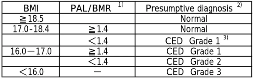
James et al, (1988) estimates the level of chronic energy deficiency by using a combination of BMI data and the energy consumption based on individual physical

(8)

activity level (PAL) (Table 1). BMI is divided into four groups (18.5 or over; 17.0-18.5; 16.0-17.0 and under 16.0). Values of 18.5 or over are considered normal. For BMI levels from 17.0 up to but not including 18.5, if the PAL is greater than or equal to 1.4, the person is also considered normal, and if the PAL is less than 1.4, the person is considered to be suffering from chronic energy deficiency２

. If the BMI is less than 17.0, the person is considered to be suffering from chronic energy deficiency regardless of the level of PAL.

4) BMI and intrahousehold resource allocation

Much empirical research has been conducted in order to elucidate the relationship between nutritional intake quantity and labor productivity. There are also cases where BMI is applied as an index to understand intrahousehold resource allocation (Dercon & Krishnan 2000:692; Pitt et al. 1990)３_{. The reason lies in the fact that measurements are}

much easier and the margin of error is smaller than when dealing with data such as consumption, nutritional intake, and income. In particular, from the viewpoint of intrahousehold resource allocation, individual BMI data is useful for obtaining information on individual family members. It is difficult for each individual to grasp their individual income and their nutritional intake accurately. Therefore, it can be maintained that BMI is valid data for each individual (Dercon and Krishnan 2000:691). In this paper, the problem of the intrahousehold resource allocation between males and females is not dealt with directly. However, the comparison between females of female-headed households and females of male-headed households implies the resource allocation to females in a family.

(9)

2. The Model of BMI

The functions of BMI can be divided into stock and flow. In the stock part, A(at-1) is used as the function of accumulated stock until t-1 period. The function of flow part as B includes the nutritional intake N(nt) and the energy consumption C(ct) during t period. The genetic factors H are constant and also included in the B. They have an influence on the efficiency of the nutritional intake and the energy consumption. We can write this equation as:

BMIt＝A(a t-1)+B[N(nt)-C(ct), Ｈ] (1)

Next, each function of equation (1) is examined. First, A (a t-1) has an equivalent value to BMI t-1 but a data set with a time series of BMI is not available in this paper. Thus, personal histories such as birthplace and education are used as the proxy variables of A (at-1).

For nutritional intake N(nt), it is assumed that the household income i is converted into nutritional intake λ. Let p (0 ≦ p ≦ 1) be the ratio of intrahousehold resource allocation to each member of the household. The equation of N(nt) is:

N(n t)＝N(λ i t･p, s t) (2)

s shows seasonality. Agricultural seasonality in income resulting in nutritional intake is taken into account, such as low nutritional intake before harvesting and high nutritional

(10)

intake in the post-harvesting period.

Considering energy consumption C (ct) as the product of the basal metabolic rate (BMR) and the physical activity level (PAL:l)４_{. The function D for BMR includes age y}

in inverse proportion, and weight w and hight h in proportion to BMR５_{. For the}

function L for PAL in developing countries, seasonality s in agriculture should be considered. In particular, the quantity of labor required during the plowing and harvest seasons is completely different from other periods. Therefore,

C(ct)＝C[D(yt, w t, h t )・L(lt, s t ) ] (3)

As for the genetic factor H, information such as the differences among ethnic groups and the physical condition of the parents and relatives is required. It is, however, difficult to distinguish only the genetic factors accurately because the socioeconomic environments are intertwined with the genetic factors. Therefore the equation of BMI will be:

BMIt＝A(a t-1)+B[N(λi t･p, s t)- C[D(yt, w t, o )・L(lt, s t )], H] (4)

3. BMI Analysis in the Amhara Region of Ethiopia

1) Outline of Ethiopia and the Amhara region

(11)

males and females because the absolute poverty of the country also causes problems. Ethiopia is one of the most seriously poverty-affected countries in the world. According to the World Bank, gross income per capita in 2002 was less than 100 dollars (World Bank 2004a:14). Therefore, since the economic pie itself is very limited, equal resource allocation among family members cannot solve the poverty itself.

Females, however, are certainly in a much harsher position than males. The risk to life they face, including from pregnancy and childbirth, is larger than that of males. In addition, the lower social position of females affects their economic situation. For instance, females’ right to inherit land is considerably restricted compared to males (World Bank 1998:16). Concerning education, although both males and females are legally given equal educational opportunities, the ratio of current school attendance and school attendance experience varies for males and females. The percentage for males is 27.5%, while for females it is lower, at 16.7%６_{(CSA 1999a:69).}

b. Female-headed households in Ethiopia

It should be noted that the proportion of female-headed households is high in Ethiopia. The ratio of female-headed households is 22% in Ethiopia overall, and 35% in urban districts (Table 2). According to the data from the World Bank (2004b:331), Ethiopia carries a relatively higher proportion of female-headed households among African countries. According to the World Bank (2004b:331), female-headed households in Ethiopia account for 18% of the total Ethiopian households (from available data for 1991-1999). Ethiopia is placed fifth among the 22 African countries with available data, with a simple mean value of 13% and a median of 13.5%.

Table 3 shows the marital status of females of 10 years of age or older, based on the results of the 1994 National Census. Most unmarried females live with their parents.

(12)

Aside from unmarried females, the reasons why females are single are divorce or the death of their husbands. Cases of divorce predominate in urban areas, while cases of widowhood are more widespread in rural areas. Regarding the Amhara region, virilocal marriage is the general pattern, and in case of separation, remaining in the virilocal area is difficult for females, so in most cases they leave the rural area and migrate to urban districts, based on case study results (Yared 1999:46-49; Teferi 1998:80-81).

c. An overview of the Amhara region and the situation of females in the region

The Ethiopian government introduced a federal system in 1994. The administrative borders of regions were decided basically by the distribution of ethnic groups. Therefore, 91% of the population in the Amhara region is Amhara (CSA 1998a:36).

The Amhara region is located in the northern central part of Ethiopia. The population is about 19 million, which represents 25% of the total national population (Central Statistical Agency 2006:24). Although Bahir Dar, the regional capital, is the most important city in Amhara, its population is 167 thousand, which represents only 0.9% of the regional population. Eighty-nine percent of this population resides in rural areas, and those engaged in agricultural and fishing activities constitute 90% of the total population (Central Statistical Agency 2006; and CSA 1998a).

In terms of the situation of females, the unique point is the high ratio of divorce cases. As Table 3 shows, the divorce rate is 14%, which is twice the nationwide average of 7% (Table 3). Several case studies also mentioned the high divorce rate in the Amhara region (Pankhurst 1992; Aspen 1993).

In addition to marital status, a land policy in 1990 in the Amhara region had a major impact on females’ land rights. In 1990 just before the socialist regime was overthrown

(13)

in 1991 by the Ethiopia People’s Revolutionary Democracy Front (EPRDF), most of the Amhara region was under the control of the EPRDF. At that time, the EPRDF carried out a land reallocation７_{. As stated in detail in Teferi (1998}₎_{, this land reallocation}

consisted of allotting a plot of land per adult, so in the case of a married couple, the land per household would be double the land allotted to a single person. Due to this allotment method, females’ right to own land, which had been prescribed by law but only nominally８_{, started to be recognized in earnest.}

In a field study carried out by the author in the rural area of the Amhara region, a married couple had acquired the land equivalent to two persons and divided it upon divorce into two halves, with each one owning his or her own plot. Divorced females, who do not normally plow the land themselves, lend it out to adult males and receive half of the crop as rent. This is a new trend because the tradition of virilocal marriage has usually caused females to leave the virilocal area without retaining any land ownership. This kind of land allotment, however, was not carried out after 1990 due to a land shortage (Kodama 2005).

2) Demographic Health Survey (DHS) data

Data used in this study is mainly from the Ethiopian Demographic Health Survey (DHS) carried out in 2000. This survey was conducted by the Central Statistical Authority (CSA) of Ethiopia with the financial aid of the United States Agency for International Development (USAID) and the United Nations Population Fund (UNFPA).

The survey covered 539 areas in the country (138 urban areas９_{, 401 rural areas).}

(14)

households were interviewed, including 15,367 females between 15 and 49 years of age and 2,607 males between 15 and 59 years of age (CSA 2000:3).

This paper used data from the Amhara region covering 1,407 females between 15 and 49 years of age, including 211 female household heads and 1,196 married females１０_.

The survey was conducted from February to May, which is the agricultural off-season period. This paper used BMI data of females who had given birth during the previous five years and who were not pregnant at that time. Furthermore, cases where the height numerical value exceeded 4.25 times or more than the standard deviation from average height were excluded１１_.

There are two limitations concerning the DHS data. First, as the survey was conducted at one single point in time, individual changes through time are not available. Second, the research gathered individual personal data, and not information concerning things such as environment or social customs surrounding the individuals. To alleviate this problem, previous anthropological research and the national census complement the DHS data.

Furthermore, in this paper, age groups in five-year spans are basically used. This is because, as shown in Figure 1, when the respondents answered about their age, in most cases they did no tell their exact age, but they replied with numbers ending in five or zero. This tendency is verified not only in DHS data but in the National Census as well (CSA 1999a:21).

Concerning the statistical analysis of sample numbers and mean values, the sample weight suggested by the DHS has been applied to correct the sampling bias.

(15)

In the previous section the model was presented. Based on equation (4), independent variables from the DHS data were selected, as Table 4 shows. Below, an explanation of each item follows.

a. Personal history

As variables related to the stock until t-1 period in equation (4), the following have been used: childhood place of residence, number of marriages, education level, number of months elapsed after childbirth. First, regarding childhood place of residence, this variable was selected as one which exerts an effect on nutritional intake during childhood. The number of marriages and the education level are effective variables for showing the wealth of the parents. This is strongly related to marriage traditions. In the case of Amhara, marriage is in most cases decided by both pairs of parents, who consider the wealth and social position of the prospective partner of their son or daughter (Hoben 1973:59). At the time of marriage, it is customary for both sets of parents to contribute equally to the new household with livestock (usually cows) or to offer the equivalent amount in cash. The preparation for the equal wealth is also required for second marriages. If a partner is not prepared to offer a similar value in property to the other partner, remarriage also becomes difficult１２_{. Therefore, the}

possibility of several remarriages shows that the bride’s parents are sufficiently wealthy. The education level is also a variable that indicates the parent’s wealth. Especially in rural areas, unlike the urban districts, access to education and literacy programs is limited and in a distant location. It is highly probable that the fact that a household can afford to send children to school despite large distances１３_{indicates the high economic}

(16)

position of the household.

Finally, the number of months elapsed from the last childbirth affords a means to take into account the weight change brought on by pregnancy. It is necessary to take this into account because during the gestation period, fat accumulates easily and as a result, weight increases considerably.

b. Nutritional intake

Regarding nutritional intake, first, the variables that may be mentioned are those related to income, such as the occupation of females, or their husbands or partners１４_,

and the number of children contributing to the household economy. Differences in marital status also indicate economic status because economic status is strongly affected by the economic contribution of husbands. In the case of married females, the age gap with husbands can be considered as a variable related to the intrahousehold resource allocation. In addition, the number of children living together in the same household also has an effect on resource allocation.

Among the variables used in equation (4), the one that expresses seasonal fluctuation has not been included in this study because the survey was carried out at one point in time, during the agricultural off-season.

c. Energy consumption

Concerning energy consumption, age is considered a variable of the basal metabolic rate. An increase in age produces a decrease in the basal metabolic rate. Therefore, if calorie intake remains atthe same level and physical exercises also remain unchanged, weight and BMI are expected to increase. The number of sons or daughters living

(17)

together in the same household affects the daily activity level because they might contribute to the labor force. In addition, in Ethiopia children are assumed to make important contributions to the reduction of housework, especially daughters, as housework is considered heavy, time-consuming work (Dejene 1995:26-27). Calorie loss by breast-feeding is also an important matter when considering energy consumption.

d. Genetic factors

DHS does not deal with variables related to genetic factors. Therefore, although their influence on BMI is clear from previous research, they are not included in this analysis. The disadvantage of omitting genetic factors should be minimal because the analysis focuses on a region where the ethnic homogeneity is high, as mentioned above.

e. Other external factors

External factors related to the social and cultural structure of the residence area (urban or rural area) and religion (Ethiopian Orthodox or Muslim) have been included as variables.

Among the variables used in this study, there are some which include biological elements not directly related to the social structure, for example "the number of months elapsed after childbirth," "breastfeeding," and "age." These variables are referred to in the analysis only when the results obtained are anomalous.

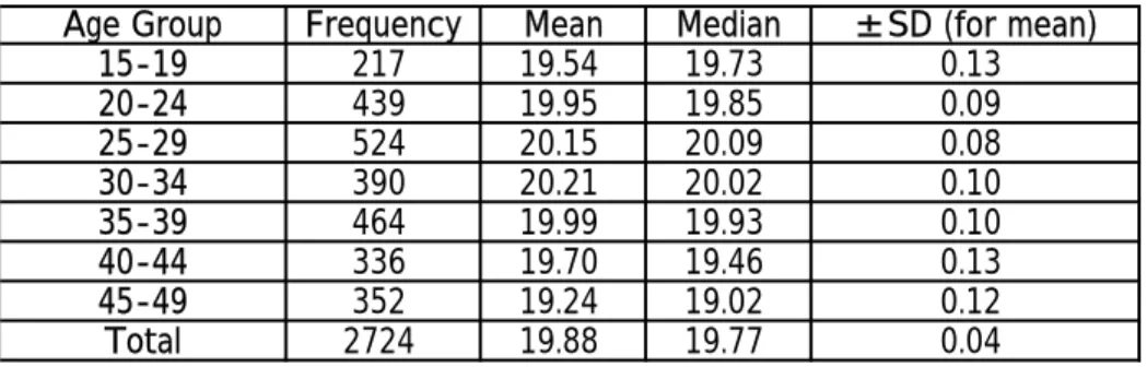
In particular, in the regression analysis for which consideration of linear functions is a prerequisite, it is difficult to reach a correct result concerning the age variable. When

(18)

changes in the mean value of each age group are considered, the shape is close to a quadratic function (Table 5 and Figure 2). BMI reaches its peak in the first half of the thirties. Then, it follows a decreasing tendency. Therefore in the regression analysis, the age group variable is included but is not an object of analysis.

4) Classification

When there are many groups with completely different social and economic structures, it is impossible to know the specific features of each group if only one general, consolidated analysis is carried out. Therefore, an appropriate group classification is critical.

Classification by residential area should be considered. Regarding the occupation ratio by residence area in the Amhara region (including those 10 years of age or older engaged in economic activity), those engaged in the agricultural or fishing industries in the rural areas amount to 97.6% (males 98.8%, females 96.1%), as contrasted with the urban districts, where the percentage is only 14.6% (males 19.0%, females 9.6%) (1994 Census, CSA 1998a). In urban districts, the occupation that engages the most males, 19.2%, is "wholesale and retail trade, car repair and daily necessity sales," while the occupation that engages the most females, 31.3%, is work in hotels and restaurants (administration/service) (CSA 1998a:133).

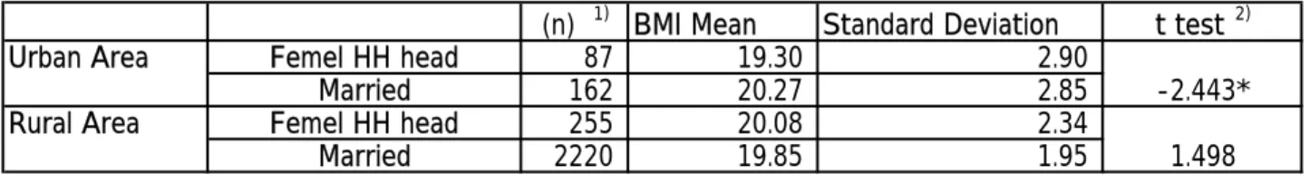
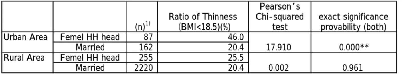
The BMI data of the DHS more obviously shows the differences by the residential area. As shown in Table 6 and Table 7, the nutritional status of married females is better than that of female household heads１５_{in urban districts, while in rural areas there is no}

(19)

there is some kind of difference in the socioeconomic structure between urban and rural areas１６_{. Below follows an analysis comparing urban and rural areas.}

5) Statistical results

a. Amhara region in total (Table 8)

Table 8 shows the results of regression analysis (OLS: Ordinary Least Squares) of the Amhara region by urban and rural areas, using the independent variables mentioned above and females’ BMI as a dependent variable.

First, the result of the regression analysis on the BMI of females in the Amhara region is considered. As the variables most affecting BMI, the standard partial regression coefficients are given in decreasing order: "professional occupation of the husband/partner," "number of daughters 10 years old or older living in the same household," single marriage or multiple and "literacy" The larger the variables, the more positive the observed influence on BMI. Therefore, the variables most affecting BMI are those related, not to the individual, but to the household situation, such as the husband’s wealth (husband’s occupation dummy), parent’s wealth (multiple remarriages), and the number of daughters who can contribute to reduction of housework.

The comparison between urban and rural areas shows several unique points. First, in the urban areas, the BMI value of married females is higher than that of female household heads, while in the rural areas, the BMI of female household heads is higher than that of married females.

(20)

engaged in a professional occupation, there is a positive effect on the BMI of females. In contrast, what affects the females’s BMI in rural areas is whether the household owns land or not.

In addition, the size of the marriage dummy and the literacy dummy, which indicate the wealth of females’ parents, also is different in urban and rural areas. The number of marriages has a major influence in urban areas, while in rural areas it is the size of the literacy dummy that has a major influence. This might show that the cost of receiving education is higher in rural areas than in urban areas.

Thus, the factors affecting the BMI in the urban and rural areas are different. In order to verify details, urban and rural areas are analyzed separately.

b. Urban areas (Table 9)

As noted above, what most affects females’ BMI in urban areas is the presence of the husband. Therefore, a comparison between married females and female household heads is critical for the analysis of urban areas. Table 9 reports the results of the regression analysis performed on each group.

(1) Female household heads in urban areas

What most affects the BMI of a female household head is the occupation of the partner who does not live together in the same household. This means that the financial help of the partner has a great influence on the female household head’s economic situation. The importance of males’ wealth can also be inferred from the results that show that the BMI of a widow is significantly lower than that of the divorced woman. This may result from the fact that the death of the husband, which implies the loss of her provider, is

(21)

frequently an abrupt, unavoidable event, so it has a greater impact on females’ nutritional intake than the case of divorce, a situation for which one can prepare.

Concerning the influence that the number of sons and daughters living outside of household has on BMI, even with a significant level at 5%, it is difficult to interpret the factors by only considering the DHS data. The results show that the more sons there are living outside of the households, the more the BMI of females decreases, while the more daughters there are living outside of the households, the more the BMI of females increases. As a provisional inference, it can be said that this is due to the fact that as long as the children remain within the same household, they receive support to continue education, but when they cease to be part of the household, the support is cut off. The school attendance rate of sons is higher than that of daughters１７_{, and so there is a}

possibility that the household is supporting a son so that he can receive higher education in a place outside his residence area. On the other hand, the marriage age of females is much lower than that of males. As most females form a new household in the second half of their teens１８

, they leave their original household earlier than males, which may imply that resource allocation to daughters becomes unnecessary. However, due to the lack of detailed profiles of children who live separately, it is difficult to reach a conclusion.

Another feature of female household heads is that the BMI of individuals from rural areas is significantly lower than those coming from urban areas. These results will be examined later with the results for rural areas.

(2) Married females in urban areas

(22)

the BMI are given as follows in decreasing order, according to the standard partial regression coefficient: "number of daughters living in the same household" and "single marriage or multiple marriages ". In other words, the parents’ wealth (number of marriages) and the reduction of domestic chores due to daughters living in the same household are the variables producing greatest impact on BMI.

In the case of the cohabitation of females other than daughters, no similar effects could be seen. A separate study about the profile of the cohabiting females (for instance, the husband’s mother or other relatives) is necessary.

c. Rural areas

The results of Table 10 as well as Table 7 indicate that the BMI of female household heads in rural areas is higher than that of married females. An exploration of the rural area follows, taking into consideration the causes which led to these results.

(1) Female household heads and married females in rural areas (Table 10)

Table 10 shows the regression results of the BMI of females in rural areas, classified in two groups: female household heads and married females.

First, concerning female household heads, the results indicate that whether her partner holds a professional post or not has the most influence on the BMI. However, as the number of samples (real number) is only one, and though statistically it is a significant result, the conclusion on this variable is reserved.

Another element to consider is the number of daughters 10 years old orolder living in the same household, which contributes to domestic chore reduction. The more daughters living together in the household, the more the BMI increases. In addition, the BMI also

(23)

increases when a household owns land. Furthermore, the high land ownership rate is a major feature of female household heads in rural areas. Considering that the land ownership ratio is 69% for households of married female in rural area, the land ownership for female household heads is still high, at 52%１９_{. This is an important}

feature because it is contrasted with female household heads in urban areas, where no cases of land ownership have been registered.

Literacy, which indicates the wealth of parents, has a great influence on married females. Regarding religion, the BMI of Muslim married females is lower than Orthodox married females. Muslims in the Amhara region might be in a more unfavorable position in terms of intrahousehold resource allocation.

(2) Landowners and non-landowners in rural areas (Table 11)

Table 11 shows the results of the comparison between landowning households and non-landowning households because in rural areas, not only the marital status, but land ownership as well affects females’ income. Table 11 classifies rural households as landowning or non-landowning, and shows the results of regression analysis on females’ BMI.

Among landowning households, the BMI is higher when there is not a husband. This is suggestive from the viewpoint of intrahousehold resource allocation. Findings of previous research also indicate that when land is owned, the female household heads are in a better situation than the married females (Original 1999:207). For instance, females who are household heads can take initiative in harvesting matters and can also participate in organizations such as peasant associations, as a representative of their own households. Moreover, in most female-headed households, females do not plow the land

(24)

by themselves, but rent it out and receive half of the crop as payment２０_{. Taking this}

fact into consideration, in the case of resource allocation in a married couple’s household, the husband receives more than a half of the total income. In the case of landowners, as the number of breadwinning sons increases, females’ BMI becomes higher.

The BMI increases, even if the land is not owned, when there is access to rented land. This means that in rural areas the access to land has a major effect on females’ BMI. In cases where the land is not owned, the existence of cohabiting females (including females other than daughters) contributes to the females’ BMI improvement.

d. Females migration from rural to urban areas

Of females living in urban areas, 68% come from rural areas. This figure includes 56% of female household heads and 72% of married females２１_{. In other words, urban and}

rural areas are not isolated from each other, as the majority of the urban area population comes from rural areas.

The migration pattern from rural to urban areas can be divided into two groups. One group is the female household heads who have no access to land, and thus migrated to the urban districts. The other group includes females who migrated for marriage to a man living in the urban districts. Particularly concerning the former, the data shows that there are no landowners among the female household heads in urban areas.

Behind the migration from rural to urban areas, there is a land shortage problem which has been getting worse. At present, the Amhara region is facing a serious land shortage (Dessalegn 1994). Under these circumstances, the existence of an unmarried man owning land in rural areas is rare. Thus, parents send their daughters to urban areas,

(25)

seeking a man with a better income.

On the other hand, if a woman who was married in a rural area did not have the opportunity to participate in the 1990 land redistribution, her possibilities to have access to land is very low. Upon divorce, females are only entitled to take their movable property (World Bank 1998:16). This explains the difficulty females have in remaining in rural virilocal areas. In some cases, females migrate to urban districts only to secure survival.

Conclusion

In this paper, female social and economic status in the Amhara region has been analyzed, using a large-scale sampling of data, focusing especially on nutritional status. The analysis focused on a 2 x 2 classification considering: urban areas/rural areas and married females/female household heads. The analysis shows that the females in the most disadvantageous situation are the female household heads in urban districts who, unlike their rural counterparts, do not have access to land ownership, nor can they count upon the support of a husband.

In order to understand the factors leading to this kind of result, it is necessary to take into account the vast differences existing between the socioeconomic structure surrounding females in the urban districts and those in rural areas. In urban districts, almost no landowners exist, and the main economic activity is not related to agriculture. In rural areas, most individuals are engaged in agricultural activities. Therefore, the factors affecting females’ economic situation differ in the urban and rural areas.

(26)

combination of a culture of male predominance and females’ low rate of school attendance results in few opportunities for females to secure an income. In other words, females cannot avoid depending on the financial power of their husbands or partners. Thus, the BMI of the female household heads, who cannot secure the constant support of a man, is lower than that of married females.

On the other hand, in the case of rural areas, ownership or lack of ownership of land has a great influence on the BMI. The results obtained in this paper also show that if a female household head owns land, her nutritional intake is higher than in the case of married females. This is because female household heads benefit more than their married counterparts in intrahousehold resource allocation, as the latter have to share resources with their husbands.

Therefore, it is difficult to simply conclude that female household heads in rural areas are in a favorable situation, without considering landownership. This is because when a woman residing in a rural area becomes a female household head, it is difficult for her to remain there; only female household heads who can afford landownership can remain in rural areas. The rest migrate to urban districts. The socioeconomic structure of rural areas pushes poor females out to urban districts. This is also supported by the fact that, in female-headed households in urban areas, the BMI of individuals who have migrated from rural areas is lower than their counterparts from urban districts (Table 9). It does not, however, mean that all the migration of females from rural areas to urban districts leads to pauperization because most married females in urban districts who enjoy a higher BMI are migrants from rural areas. Urban districts offer different options for females coming from rural areas.

(27)

References

Alderman, Harold［1993］ New Research on Poverty and Malnutrition: What Are the Implications for Policy? in Michael Lipton and Jacques van der Gaag, Including the Poor, Washington, D.C.: World Bank, pp.115-131.

Appleton, Simon and Paul Collier［1995］ On Gender Targeting of Public Transfers, in van de Walle, Dominique and Kimberly Nead eds., Public Spending and the Poor : Theory and Evidence, London : Johns Hopkins University Press, pp.555-581.

Aspen, Harald [1993] Competition and Co-operation North Ethiopian Peasant Household and their Resource Base,s Trondheim, University of Trondheim.

c

o c

e

Bardhan, Pranab and Christpher Udry [1999] Development Microe onomics, New York and Oxford: Oxford University Press.

Befekadu Degefe, Berhanu Nega and Getahun Tafesse［2002］Second Annual Report on the Ethiopian Economy: Volume II 2000/2001, Addis Ababa: Ethiopian Economic Association.

Bureau of Rural Development［2003］Rural H useholds Socio-E onomic Baseline Survey of 56 Woredas in the Amhara R gion Volume III - Education, Bahir Dar: The Federal Democratic Republic of Ethiopia, Amhara National Regional State. Central Statistical Agency [2006] Ethiopia: Statistical Abstract 2005, Addis Ababa:

Central Statistical Agency.

Central Statistical Authority（CSA）［1998a］The 1994 Population and Housing Census of Ethiopia: Results for Amhara, Volume II, Statistical Report, Addis Ababa: CSA.

(28)

Volume II, Statistical Report, Addis Ababa: CSA.

――［1998c］The 1994 Population and Housing Census of Ethiopia: Results for Tigray Region, Volume II, Statistical Report, Addis Ababa: CSA.

――［1998d］The 1994 Population and Housing Census of Ethiopia: Results for Southern Nations, Nationalities and Peoples’ Region, Volume II, Statistical Report, Addis Ababa: CSA.

――［1998e］The 1994 Population and Housing Census of Ethiopia: Results for Tigray, Volume II, Statistical Report, Addis Ababa: CSA.

――［1999a］The 1994 Population and Housing Census of Ethiopia: Results at Country Level, Volume II, Analytical Report, Addis Ababa: CSA.

――［1999b］The 1994 Population and Housing Census of Ethiopia: Results for Addis Ababa, Volume II, Analytical Report, Addis Ababa: CSA.

――［1999c］The 1994 Population and Housing Census of Ethiopia: Results for Affar Region, Volume II, Analytical Report, Addis Ababa: CSA.

――［1999d］The 1994 Population and Housing Census of Ethiopia: Results for Benishangul-Gumuz Region, V lume II, Analytical Reporto , Addis Ababa: CSA. ――［1999e］The 1994 Population and Housing Census of Ethiopia: Results for Dire

Dawa Provisional Administration, Volume II, Analytical Report, Addis Ababa: CSA.

――［1999f］The 1994 Population and Housing Census of Ethiopia: Results for Gambella Region, Volume II, Analytical Report, Addis Ababa: CSA.

――［1999g］The 1994 Population and Housing Census of Ethiopia: Results for Harari Region, Volume II, Analytical Report, Addis Ababa: CSA.

――［1999h］The 1994 Population and Housing Census of Ethiopia: Results for Somali Region, Volume II, Analytical Report, Addis Ababa: CSA.

(29)

Dejene Aredo［1995］The Gender Division of Labour in Ethiopian Agriculture: A Study of Time Allocation among People in Private and Co-Operative Farms in Two Villages, Addis Ababa: Organization for Social Science Research in Eastern and Southern Africa（OSSREA）.

Dercon, Stefan and Pramila Krishnan［2000］ In Sickness and in Health: Risk Sharing within Households in Rural Ethiopia, Journal of Political Economy, Vol.108, No.4, Aug.2000, pp.688-727.

Dessalegn Rahmato ed.［1994］Land Tenure and Land Policy in Ethiopia After Derg, Trondheim: University of Trondheim.

Frankenfield, D.C., W.A.Rowe, J.S.Smith, and R.N.Cooney [2003], “Validation of Several Established Equations for Resting Metabolic Rate in Obese and Nonobese People”, Jou nal of the American Dietetic Association, Volume 103, No.9, September 2003, pp.1152-1159.

r

Gamohara, Seika[1998b] Himan Idenshi (Obese Gene in Japanese), Tokyo: Koudansha. Hoben, Allan［1973］Land Tenure among the Amhara of Ethiopia: The Dynamics of

Cognatic Descent, Chicago and London: University of Chicago Press.

James, W.P.T., A.Ferro-Luzzi and J.C.Waterlow［1988］ Definition of Chronic Energy Deficiency in Adults: Report of a Working Party of the International Dietary Energy Consultative Group Discussion Paper, European Journal of Clinical Nutrition, 42, pp.969-981.

Kodama, Yuka [2005] “The Challenge of Land Tenure System and Gender Issues in Ethiopia: A Case of Land Reform Policy in the Amhara Region”(in Japanese) Africa Report, No.40, March 2005.

Meier, Gerald, M. and James E. Rauch［2000］Leading Issues in Economic Development, Seventh Edition, New York and Oxford: Oxford University Press.

(30)

through Sustainable Land Use: Policy on Institutional, Land Tenure, and Extension Issues in E hiopia, Addis Ababa: NOVIB Partners Forum on Sustainable Land Use, 1999, 203-213.

t

s

c

Pankhurst, Helen［1992］Gender, Development and Identity: An E hiopian Study, London and New Jersey: Zed Books.

Pitt, Mark M., R.Rosensweig and Md.Nazmul Hassan［1990］ Productivity, Health, and Inequality in the Intrahousehold Distribution of Food in Low-Income Countries, The American Economic Review, Vol.80, No.5, Dec, pp.1139-1156. Scrimshaw, N.S., J. C. Waterlow and B. Schürch et al [1996] Energy and Protein

requirement , Proceedings of an IDECG workshop, Hampshire, Stockton Press ( The document can be retrieved through

http://www.unu.edu/Unupress/food2/UID01E/uid01e00.htm).

Sen, Amartya［1995］ The Political Economy of Targeting, in Dominique van de Walle and Kimberly Nead, eds., Public Spending and the Poor : Theory and Evidence, London: Johns Hopkins University Press, pp.11-24.

Strauss John and Duncan Thomas ［ 1998 ］ Health, Nutrition and Economic Development, Journal of E onomic Literature, Vol.36, No.2, June, pp.766-817. Teferi Abate［1998］Land, Capital and Labour in the Social Organization of Farmers: A

Study of Household Dynamics in South-western Wollo, 1974-1993, Addis Ababa: Department of Sociology and Social Administration, Addis Ababa University. World Bank ［ 1998 ］Implementing the Ethiopian National Policy for Women:

Institutional and Regulatory Issues, Washington, D.C.: World Bank.

――［2004a］World Development Indicators 2004, Washington, D.C.: World Bank. ――［2004b］African Development Indicators 2004, Washington, D.C.: World Bank. World Health Organization（WHO）［1986］ Use and Interpretation of Anthropometric

(31)

pp.924-941.

Yared Amare［1999］Household Resources, Strategies and Food Security in Ethiopia: A Study of Amhara Hou ehold in Wodga, No thern Shewa, Addis Ababa: Department of Sociology and Social Administration and The Addis Ababa University Press.

s s r

１_{This is connected to the discussion on targeting of aid. Targeting is utilized in cases in which} aid funds are limited, where, the target is more focused in order to raise efficiency. On the other hand, much discussion has taken place concerning the efficiency of targeting (Sen 1995). ２_{A PAL of 1.4 is “the realistic maintenance requirement for sedentary people” (James, et al.}

1988:970).

３_{In Pitt et al. (1990), BMI is not used, but the research on intrahousehold resource allocation} in Brazil uses weight/height data.

４_{Concerning the physical activity level index (PAL), see Scrimshaw, et al. (1996) for the} detailed classification.

５

Based on the Harris-Benedict equation. Although it is widely used for estimating BMR, some recent studies have pointed out the inaccuracy (Frankenfield, et al, 2003 ).

６_{Percentage of 5-year-old and older population attending school or having attended} school (figures for the whole country).

７_{However, since according to the Constitution, land is government-owned, this is a right to the} use of land. In this paper, for the sake of convenience, the possession of the right to the use of land is referred to as “land ownership”.

８_{According to the Amhara customary law, it is assumed that males and females have equal} rights at the time of succession, but in real life, land is inherited almost exclusively by males (World Bank 1998:16-22).

９_{The urban areas include "big cities" (the capital city and cities with a population of one} million or more), “small cities” (population of 50,000 up to one million) and towns (other urban districts) (DHS, Description of the Demographic and Health Surveys: Individual

Recode Data File, DHSIII, Version 1.1, 2004).

１０_{In some usages, female-headed households include households with husbands or partners} living together. However in this paper, for the sake of considering the intrahousehold resource

(32)

allocation, the classification of “married females” refers to cases where husbands or partners live in the same household, while “female-headed households” ·includes cases where no husband or partner lives in the same household.

１１

Values that were markedly different in each group were rejected based on the Smirnov-Grubbs outlier test at 1% significance level (one-sided).

１２_{Based on a field survey carried out by author in July 2003.}

１３_{For instance, the walking distance from home to the elementary school in rural areas in the} Amhara region is 2.6 hours on average (Bureau of Rural Development 2003:25).

１４_{A partner who does not live in the same household implies a relationship with economic aid} from the partner, rather than a mere casual relationship. In most cases, the term “partner” refers to cases of relationships with married males (according to the field survey carried out by author in July 2003). Therefore, the economic strength of the partner affects the economy of the female-headed household.

１５_{Female-headed households dealt with in this paper are limited only to those cases where} such households were established upon the divorce or death of the husband. Female-headed households of unmarried females were not considered in this analysis because only four samples were available.

１６_{Even the perception of obesity is different in urban and rural areas. In rural areas or small} cities in the Amhara region, being fat is preferred to being thin. However, in Bahir Dar, the regional capital, more females perceived thinness as better than fat (according to the field survey carried out by author in February 2004).

１７_{In the Amhara region, the schooling experience rate for males is 22% and for females is} 12% (CSA 1998a:57).

１８_{For instance, according to the 1994 National Census, the percentage of married people} between 15 and 19 years of age living in the Amhara region was 41% for females and 9% for males (CSA 1998a:30).

１９_{Sample weight adjustments were applied.} ２０

Based on a field study carried out by author in 1998.

(33)

Table 1 Sequential Assessment for the Epidemiological Diagnosis of Different Grades of Chronic Energy Deficiency.

BMI PAL/BMR １） Presumptive diagnosis 2)

≧18.5 Normal 17.0-18.4 ≧1.4 Normal ＜1.4 CED Grade 1 3) 16.0−17.0 ≧1.4 CED Grade 1 ＜1.4 CED Grade 2 ＜16.0 − CED Grade 3 Notes:

1) PAL: Physical activity level, BMR:Basal metabolic rate

2) For confirmation of the diagnosis and for use in clinical research it is necessary to measure individual BMRs in groups to allow for the appreciable interindividual variability. In cases of BMIs above 18.5 or below 16.0 the diagnoses can be based on the BMI values alone.

3) CED: Chronic energy deficiency

(34)

Table 2 The Ratio of Female Household Heads (over 15 years old)

Region Total Urban Rural

Tigray 31% 50% 27% Afar 14% 26% 12% Amhara 21% 42% 19% Oromiya 22% 33% 20% Somali 18% 24% 17% Benishangul-Gumuz 19% 27% 18% SNNP 22% 28% 21% Gambella 18% 26% 16% Harari 29% 38% 15% Dire Dawa 27% 32% 15% Addis Ababa 33% NA NA Ethiopia total 22% 35% 20% Source: CSA[1998a∼e][1999a∼h]

(35)

Table 3 Marital Status (females over 10 years old ) National Amhara Region

Total Urban Rural Total Urban Rural

Married 49.4 32.4 52.6 52.9 31.3 55.6

Unmarried 35.4 47.3 33.1 25.6 39.7 23.8

Divorce 6.9 11.7 5.9 13.8 20.7 12.9

Widow 8.1 8.2 8.1 7.5 8.0 7.4

Others 0.3 0.3 0.3 0.3 0.4 0.3

(36)

Figure 1: Age Distribution of Females in the Amhara Region (15-29 year old) 0 20 40 60 80 100 120 140 15 16 17 18 19 20 21 22 23 24 25 26 27 28 29 30 31 32 33 34 35 36 37 38 39 40 41 42 43 44 45 46 47 48 49 Age Source: DHS Frequencies（Weighted）

(37)

Table 4 Variables Used in the Regression Analysis of BMI.

Variables Definition

Personal History Childhood place of residence Months after child delivery

Number of marriage (once or more than once) Nutrition Intake

Income Occupation（agriculture, professionals, no employment）2) Occupation of husband/partner（agriculture, professionals）2) Education (literate/illiterate)

Income from children=(number of children (sons/daughters), (living together/separate)

Intrahousehold Allocation Marital status（married, divorced, widowed） Age difference from husband

Resource allocation to children (sons/daughters, living together/separate)

Nutrition Consumption

Basic Metabolic Rate 1) Age(in five-year spans)

Physical Activity Level Occupation（agriculture/non agriculture, no employment)2) Labor supplied from children= Number of children living together Number of females who can work

Others Breastfeeding

Other outside factors Residence (urban/rural)

Religion (Ethiopian Orthodox/ Muslims)

Notes:

1) Weight is not used as a variable although it affects on the basic metabolic rate because BMI itself is from the result of the weight divided by the square of height.

(38)

Table 5 The Changes in BMI by Age Group

Age Group Frequency Mean Median ±SD (for mean)

15-19 217 19.54 19.73 0.13 20-24 439 19.95 19.85 0.09 25-29 524 20.15 20.09 0.08 30-34 390 20.21 20.02 0.10 35-39 464 19.99 19.93 0.10 40-44 336 19.70 19.46 0.13 45-49 352 19.24 19.02 0.12 Total 2724 19.88 19.77 0.04 Source: DHS data

Figure ２ The Changes of BMI Average by Age Group

18.60 18.80 19.00 19.20 19.40 19.60 19.80 20.00 20.20 20.40 15-19 20-24 25-29 30-34 35-39 40-44 45-49 Age Group Source: DHS data BMI

(39)

Table 6 Comparison of BMI Average

(n) 1) BMI Mean Standard Deviation t test 2)

Urban Area Femel HH head 87 19.30 2.90

Married 162 20.27 2.85 -2.443*

Rural Area Femel HH head 255 20.08 2.34

Married 2220 19.85 1.95 1.498

1) Weighted by DHS specified number 2) Not assuming equal variances * 5% significance level

(40)

Table 7 Comparison of the Ratio of Thinness（BMI<18.5） (n)1) Ratio of Thinness （BMI<18.5)(%) Pearson s Chi-squared test exact significance provability (both)

Urban Area Femel HH head 87 46.0

Married 162 20.4 17.910 0.000**

Rural Area Femel HH head 255 25.5

Married 2220 20.4 0.002 0.961

Notes:

1) Weighted by DHS specified number ** 1% significnace level

(41)

Table 8 Regression Results for BMI of females in the Amhara Region(OLS)

Dependent Variable: BMI Amhara Region tot Urban Area Rural Area

Weighted count(actual number） 2722(1378) 249(112) 2473(1266) SPRC ｔ value SPRC ｔ value SPRC t value

constant 20.578 54.719** 17.025 13.210** 21.370 44.548**

INDEPENDENT VARIABLES Personal History

childhood place of residence

rural dummy (urban=0,rural=1) -0.019 -0.810 -0.043 -0.618 -0.031 -1.328 marriage dummy（times of marriage

once=0, more than once＝1） 0.058 2.801** 0.252 3.382** 0.036 1.681

literate=1） 0.057 2.748** 0.111 1.573 0.048 2.278*

months after last pregnancy -0.071 -2.608** 0.235 2.731** -0.130 -4.592**

Nutrition Intake[related to income]

land ownership dummy3) 0.055 1.757 0.057 0.859 0.064 2.031*

rental land dummy 0.032 1.332 0.015 0.230 0.041 1.583

husband/partner occupation

professional dummy（professional=1） 0.069 2.987** 0.263 3.522** 0.022 0.848 professional dummy(professional=1) 0.043 1.833 0.082 1.118 0.030 1.045 # of sons more than 10 years old in

household 0.019 0.806 0.020 0.248 0.024 0.945

# of daughters more than 10 years

old in household 0.063 2.754** 0.183 2.427* 0.029 1.215 # of sons more than 10 years old

outside of household 0.000 -0.006 -0.052 -0.768 0.010 0.397 # of daughters more than 10 years

old outside of household -0.021 -0.888 0.160 1.991* -0.029 -1.170 marriage dummy（female household

head=0、married with husband=1） 0.001 0.047 0.377 4.859** -0.057 -2.589**

Nutrition Consumption[Related to BMR and Physical Activity Level] Age group（15∼49yr old, by 5 year

old group） -0.073 -1.986* -0.082 -0.676 -0.071 -1.847* # of sons more than 10 years old in

household(same as above) - - -

-# of daughters more than 10 years

old in household(same as above) - - -

-# of females who can work aged 15-29 yr old other than the female and

daughters 0.007 0.345 -0.201 -2.655** 0.038 1.786

No job dummy（No job=1） -0.040 -1.522 -0.094 -1.337 -0.027 -0.956 land ownership dummy(same as

above)3) - - -

-rental land dummy(same as above) - - -

-Breastfeeding dummy -0.084 -3.325** 0.067 0.833 -0.107 -4.051**

Other External Factor

residence: urban dummy(rural=0,

urban=1） -0.026 -1.062 - - -

-religion：Muslim dummy (Ethiopian

orthodox=0, Muslim=1） -0.027 -1.344 0.053 0.779 -0.036 -1.701

Ｆ value 5.142** 4.205** 5.323**

Adjusted R square 0.030 0.207 0.033

Note: * significant level at 5%, ** significant at 1%. Source: DHS data

(42)

Table 9 Regression Results for BMI of Females in Urban Area in the Amhara Region (OLS)

Dependent Variable: BMI Urban Area total Female HH Head Married

Constant 17.025 13.210** 17.689 10.314** 19.484 11.000**

Personal History

childhood place of residence: rural

dummy (urban=0,rural=1) -0.043 -0.618 -0.323 -2.956** -0.032 -0.316 marriage dummy（times of marriage

once=0, more than once＝1） 0.252 3.382** 0.021 0.146 0.348 4.040**

literate=1） 0.111 1.573 0.036 0.354 0.163 1.871

months after last pregnancy 0.235 2.731** -0.206 -1.493 0.381 3.330** widow dummy(divorce=0、widow=1、

only for female HH head) -0.565 -4.292** -

-Nutrition Intake[related to income]

land ownership dummy3) 0.057 0.859 - 1) - 0.036 0.434

rental land dummy 0.015 0.230 -0.138 -1.359 - 1)

-husband/partner occupation

professional dummy（professional=1） 0.263 3.522** 0.541 4.992** 0.149 1.501 professional dummy (professional=1) 0.082 1.118 - 1) - 0.080 0.832 # of sons more than 10 years old in

household 0.020 0.248 -0.231 -1.996 0.037 0.340

# of daughters more than 10 years old

in household 0.183 2.427* -0.020 -1.171 0.353 3.655**

# of sons more than 10 years old

outside of household -0.052 -0.768 -0.278 -2.545 0.017 0.194 # of daughters more than 10 years old

outside of household 0.160 1.991* 0.445 3.700** -0.024 -0.219 marriage dummy（female household

head=0、married with husband=1） 0.377 4.859** - - -

-Age difference from husband(only for

married females) - - - - 0.119 1.545

Nutrition Consumption[Related to BMR and Physical Activity Level] Age group（15∼49yr old, by 5 year

old group） -0.082 -0.676 0.383 2.322* -0.264 -1.678*

# of sons more than 10 years old in

-# of daughters more than 10 years old

in household(same as above) - - -

-# of females who can work aged 15-29 yr old other than the female and

daughters -0.201 -2.655** -0.257 -2.410* -0.120 -1.214

No job dummy（No job=1） -0.094 -1.337 -0.086 -0.857 -0.030 -0.360

above)3) - - -

-Breastfeeding dummy 0.067 0.833 -0.213 -1.535 0.068 0.625

Other External Factor

urban=1） - - -

orthodox=0, Muslim=1） 0.053 0.779 -0.323 -2.832** 0.084 1.023

Ｆ value 4.205** 4.374** 4.099**

Notes: 1) No sample

(43)

Table 10: Regression Results for BMI of Females in Rural Area in the Amhara Region(OLS)

Dependent Variable: BMI Rural Area total Female HH head Married

Constant 21.370 44.548** 21.780 15.096** 21.076 40.308**

Personal History

dummy (urban=0,rural=1) -0.031 -1.328 -0.081 -1.168 -0.030 -1.210 marriage dummy（times of marriage

once=0, more than once＝1） 0.036 1.681 0.108 1.495 0.034 1.492 literate dummy（illiterate=0, literate=1） 0.048 2.278* 0.054 0.760 0.049 2.209* months after last pregnancy -0.130 -4.592** 0.047 0.517 -0.151 -5.166** widow dummy(divorce=0、widow=1、

only for female HH head) - - 0.014 0.205 -

land ownership dummy3) 0.064 2.031* 0.185 2.199* 0.038 1.077

rental land dummy 0.041 1.583 0.046 0.709 0.031 1.105

husband/partner occupation

professional dummy（professional=1） 0.022 0.848 0.145 2.278* -0.012 -0.414 professional dummy(professional=1) 0.030 1.045 - 1) - 0.056 1.747 # of sons more than 10 years old in

household 0.024 0.945 -0.120 -1.691 0.051 1.883

in household 0.029 1.215 0.151 2.130* 0.012 0.460

# of sons more than 10 years old

outside of household 0.010 0.397 0.118 1.605 -0.008 -0.309 # of daughters more than 10 years old

outside of household -0.029 -1.170 -0.035 -0.459 -0.027 -1.028 marriage dummy（female household

head=0、married with husband=1） -0.057 -2.589** - - - -Age difference from husband(only for

married females) - - - - 0.018 0.800

Nutrition Consumption[Related to BMR and Physical Activity Level] Age group（15∼49yr old, by 5 year old

group） -0.071 -1.847* -0.158 -1.477 -0.064 -1.569

-# of daughters more than 10 years old

in household(same as above) - - -

-# of females who can work aged 15-29

yr old other than the female and 0.038 1.786 0.093 1.419 0.032 1.385 No job dummy（No job=1） -0.027 -0.956 -0.048 -0.618 -0.032 -0.995

above)3) - - -

-Breastfeeding dummy -0.107 -4.051** -0.094 -1.187 -0.112 -4.087** Other External Factor

urban=1） - - -

orthodox=0, Muslim=1） -0.036 -1.701 0.028 0.423 -0.050 -2.214*

Ｆ value 5.323** 2.236** 5.013**

Notes: 1) No sample

* significant level at 5%, ** significant at 1%. Source: DHS data

(44)

Table 11: Regression Results for BMI of Females in Rural Area in the Amhara Region by Land Ownership (OLS)

Dependent Variable: BMI Rural Area Total No Land Land Owner

Constant 21.370 48.580** 19.575 28.033** 22.857 32.835**

Personal History

dummy (urban=0,rural=1) -0.031 -1.339 -0.037 -0.855 -0.037 -1.467 marriage dummy（times of marriage

once=0, more than once＝1） 0.038 1.756 0.089 2.316* 0.028 1.099 literate dummy（illiterate=0, literate=1） 0.047 2.249* 0.022 0.576 0.068 2.692** months after last pregnancy -0.127 -4.538** -0.123 -2.504* -0.143 -4.097** widow dummy(divorce=0、widow=1、only

for female HH head) - - -

land ownership dummy3) 0.064 2.033* - - -

-rental land dummy 0.039 1.515 0.125 2.579* -

-husband/partner occupation professional

dummy（professional=1） 0.022 0.834 -0.031 -0.598 0.037 1.478 professional dummy(professional=1) 0.029 1.027 0.072 1.283 - 1) -# of sons more than 10 years old in

household 0.030 1.197 -0.063 -1.370 0.063 2.076*

# of daughters more than 10 years old in

household 0.033 1.413 0.094 2.183* 0.019 0.669

# of sons more than 10 years old outside

of household 0.013 0.545 -0.072 -1.706 0.051 1.739

outside of household -0.024 -0.983 -0.048 -1.092 -0.022 -0.732 marriage dummy（female household

head=0、married with husband=1） -0.058 -2.623** 0.051 1.238 -0.104 -3.983** Age difference from husband(only for

married females) - - -

-Nutrition Consumption[Related to BMR and Physical Activity Level]

group） -0.090 -2.456* 0.081 1.146 -0.141 -3.051**

-# of daughters more than 10 years old in

-# of females who can work aged 15-29