トップ - アジア経済研究所学術研究リポジトリ ARRIDE

The contribution of supply and demand shifts

to earnings inequality in urban China

著者

Asuyama Yoko

権利

Copyrights 日本貿易振興機構（ジェトロ）アジア

経済研究所 / Institute of Developing

Economies, Japan External Trade Organization

(IDE-JETRO) http://www.ide.go.jp

journal or

publication title

IDE Discussion Paper

volume

177

year

2008-10-01

INSTITUTE OF DEVELOPING ECONOMIES

IDE Discussion Papers are preliminary materials circulated

to stimulate discussions and critical comments

Keywords: urban China, earnings inequality, inequality decomposition

JEL classification: D31, J31

* Poverty Alleviation and Social Development Studies Group, Inter-disciplinary

Studies Center, IDE ([email protected])

IDE DISCUSSION PAPER No. 177

The Contribution of Supply and

Demand Shifts to Earnings

Inequality in Urban China

Yoko ASUYAMA*

Abstract

This paper examines the degree to which supply and demand shift across skill groups contributed to the earnings inequality increase in urban China from 1988 to 2002. Product demand shift contributed to an equalizing of earnings distribution in urban China from 1988 to 1995 by increasing the relative product for the low educated. However, it contributed to enlarging inequality from 1995 to 2002 by increasing the relative demand for the highly educated. Relative demand was continuously higher for workers in the coastal region and contributed to a raising of interregional inequality. Supply shift contributed essentially nothing or contributed only slightly to a reduction in inequality. Remaining factors, the largest disequalizer, may contain skill-biased technological and institutional changes, and unobserved supply shift effects due to increasing numbers of migrant workers.

The Institute of Developing Economies (IDE) is a semigovernmental,

nonpartisan, nonprofit research institute, founded in 1958. The Institute

merged with the Japan External Trade Organization (JETRO) on July 1, 1998.

The Institute conducts basic and comprehensive studies on economic and

related affairs in all developing countries and regions, including Asia, the

Middle East, Africa, Latin America, Oceania, and Eastern Europe.

The views expressed in this publication are those of the author(s). Publication does not imply endorsement by the Institute of Developing Economies of any of the views expressed within.

INSTITUTE OF DEVELOPING ECONOMIES (IDE), JETRO

3-2-2, WAKABA,MIHAMA-KU,CHIBA-SHI

CHIBA 261-8545, JAPAN

©2008 by Institute of Developing Economies, JETRO

No part of this publication may be reproduced without the prior permission of the IDE-JETRO.

The Contribution of Supply and Demand Shifts

to Earnings Inequality in Urban China

*

Yoko Asuyama

†

Institute of Developing Economies

October 2008 (Revised in June 2009)

Abstract

This paper examines the degree to which supply and demand shift across skill groups contributed to the earnings inequality increase in urban China from 1988 to 2002. Product demand shift contributed to an equalizing of earnings distribution in urban China from 1988 to 1995 by increasing the relative demand for the low educated. However, it contributed to enlarging inequality from 1995 to 2002 by increasing the relative demand for the highly educated. Relative demand was continuously higher for workers in the coastal region and contributed to a raising of interregional inequality. Supply shift contributed essentially nothing or contributed only slightly to a reduction in inequality. Remaining factors, the largest disequalizer, may contain skill-biased technological and institutional changes, and unobserved supply shift effects due to increasing numbers of migrant workers.

Keywords: urban China, earnings inequality, inequality decomposition

JEL classification: D31, J31

*

This paper is a part of the author’s thesis for the degree of Master of Public Administration at Cornell University. I thank Professor Gary S. Fields for his insightful comments and continuous guidance on my research. I would also like to thank Professor John DiNardo at the University of Michigan, and Professor Xuejun Liu at Peking University for providing me with guidance on the estimation method for supply and demand effects. I acknowledge the Research Center for Income Distribution and Poverty (RCIDP), Beijing Normal University (BNU), and the Inter-university Consortium for Political and Social Research (ICPSR), which distribute the Chinese Household Income Project (CHIP) datasets and who permitted me to use the datasets for my analysis. I would like to thank Dr. Deng Quheng at RCIDP, who helped me obtain the 2002 CHIP data quickly and interpret them appropriately. I would also like to thank Hiroko Uchimura, Shuang Zhang, and Jill Tibbett. Finally, I am grateful to the many people at IDE-JETRO who have continuously supported my life as an IDE research fellow at Cornell University. All errors are my own.

†

Poverty Alleviation and Social Development Studies Group, Inter-disciplinary Studies Center, IDE ([email protected])

1. Introduction

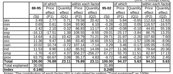
Asuyama (2008) showed how the causes of earnings inequality changed between the two periods 1988-1995 and 1995-2002 by primarily reflecting labor-related institutional reform in China. Since my analysis in this paper is an extension of Asuyama (2008) and uses the same dataset, I first reproduce here a summary of the findings in Asuyama (2008). By examining the individual samples from 1988, 1995, and 2002 of urban Chinese residents, drawn from the survey called the Chinese Household Income Project (CHIP), Asuyama (2008) first confirmed that earnings inequality in urban China continuously increased from 1988 to 2002, even when adjusted for regional price differences (RPD). The Gini coefficient based on RPD-adjusted earnings was 0.233 in 1988, 0.278 in 1995, and 0.330 in 2002, respectively. The paper then reveals how the causes of earnings inequality changed between the two periods 1988-1995 and 1995-2002 by reflecting labor-related institutional reform in China. Contrary to the situation from 1988 to 1995, between 1995 and 2002, employment status (permanent or temporary worker, etc.) became the largest disequalizer, and the decline of inter-provincial inequality contributed to a reduction in the overall earnings inequality. Individual ability, represented by education and occupation, received much greater rewards. Throughout the period from 1988 to 2002, a large part of the explained inequality increase was due to price change (changes in the valuation of individual attributes) and not due to quantity change (changes in the composition of individual attributes). Table 1 and Table 2, drawn from Tables 5-7 of Asuyama (2008) summarize these inequality decomposition results.

Asuyama (2008) argued that the above decomposition results mainly reflected labor-related institutional reform in China. However, since this reform introduced market mechanisms into the Chinese labor system, it is also necessary to examine how much supply and demand shifts contributed to the earnings inequality increase in urban China, in addition to examining institutional factors. It is possible that widening earnings differentials among education groups is due to the relative demand increase for highly educated workers, as seen in

the US. Also, supply and demand shift may have contributed to the changes in inter-provincial and intra-provincial inequality.

Numerous studies have been carried out on the causes of the earnings inequality increase in the US after 1980. There are three major explanations for the causes of rising overall inequality (or the growing educational wage differentials, which is the most important factor in the rising overall inequality). Katz and Autor (1999) label these the SDI (supply-demand-institution) explanation or framework. First, the explanation from the supply-side is that the relative supply increase in highly educated workers is considered to have contributed to a suppression of the relative wage increase to highly educated workers and thus to a reduction in inequality. However, the shrinking cohort size of the highly educated and increased numbers of unskilled immigrants may have contributed to an increase in inequality. Second, the demand increase for highly educated workers, which exceeded the supply increase of those workers, was considered one of the major factors in the rise in the relative wage of the highly educated. Product demand shift due to the increased imports of goods produced by unskilled labor and skill-biased technological change, such as the increased use of computers in workplaces, were considered the two major causes of the relative demand increase for the highly educated. Such relative demand increase for the highly educated led to the increase in the educational wage differentials. Third, institutional factors such as the decline in unionization and real minimum wage rates were also considered to be contributors to the increase in the educational earnings differentials.

There are almost no studies which estimate the degree to which supply and demand factors contributed to earnings inequality in urban China. Although, as in the US, a rising return to education in urban China has also been observed by many studies, the causes have not yet been fully investigated. For example, Zhang, Zhao, Park, and Song (2005) showed that the rising return to education in urban China from 1988 to 2001 was strongly associated with the market-oriented reform of labor market institutions. However, they also admitted that “additional work is necessary to evaluate the contributions of skill-biased technical change and

globalization to the rising returns to skill in China.” One exception is Liu, Park, and Zhao (2007), who in an “incomplete and preliminary” paper directly applied the method of Bound and Johnson (1992) to decompose wage differentials between education groups in urban China from 1990 to 2001 into five effects: 1) changes in industrial wage rents, 2) supply shift, 3) product demand shift, 4) general technological change, and 5) a residual factor. Following the method of Bound and Johnson (1992), they estimated these five effects by constructing 24 sex-education-experience skill groups.1

In this paper, I examine the degree to which supply and demand shift across skill groups contributed to the earnings inequality increase in urban China from 1988 to 2002. The major differences in my analysis from that of Liu, Park, and Zhao (2007) are as follows: First, instead of decomposing the earnings differentials between education groups as they did, I aim to measure how much supply and demand shifts across skill groups contributed to the inequality increase in the entire earnings distribution in urban China. Second, in order to take into account the existence of labor market segmentation by province in urban China, I construct skill groups by region (whether coastal or inland), education, and experience, using region instead of sex. Third, I also incorporate the supply and demand shift effects across skill groups into the inequality decomposition result presented in Asuyama (2008). As a result, I am able to present a more comprehensive picture of the causes of earnings inequality in urban China.

This paper is organized as follows: Section 2 briefly explains the dataset used in my analysis. Section 3 describes the empirical strategy by which the supply and demand shift effects are estimated. Section 4 presents the estimation results. It shows the degree to which supply and demand shift across skill groups contributed to earnings inequality in urban China. Section 4 also decomposes the total earnings inequality into supply and demand shift effects and other factors. Section 5 discusses the interpretation of the results. Finally, Section 6 summarizes the findings and mentions the limitations of my analysis.

1

After completing my analysis, I found their revised paper, Liu et al. (2008). However, their main findings are not changed largely except that they newly found that the supply shifts contributed to enlarging the wage differentials between senior and junior high school graduates in the late 1990s.

2. Data

The same dataset as used in Asuyama (2008) is used here. It contains individual samples of urban Chinese residents from 1988, 1995, and 2002, drawn from the survey called the Chinese Household Income Project (CHIP) (Griffin & Zhao, 1993; Riskin, Zhao, & Li, 2000; RCIDP).2 My sample includes only working or employed individuals who are age 16 or

above, are reporting positive earnings, and are living in the urban areas of ten provinces, namely Beijing, Shanxi, Liaoning, Jiangsu, Anhui, Henan, Hubei, Guangdong, Yunnan, and Gansu. The sample largely excludes rural-urban migrants who have rural registration (hukou) but are living in urban areas.3 Earnings are defined as annual wage, which includes bonuses and subsidies

from the primary work unit. They are adjusted for regional price differences (RPD) based on the 1988 Beijing price level. For more information on the dataset, including the treatment of missing values and summary statistics, refer to Section 2 of Asuyama (2008).

3. Empirical Strategy

I applied the methods used in DiNardo, Fortin, and Lemieux (1996) and Bound and Johnson (1992) in order to estimate the effects of supply and demand (S&D) shifts across different skill groups on their earnings change in the two periods 1988 to 1995 and 1995 to 2002.4 I briefly explain the estimation method below. For more detail, refer to the two papers

2

I acknowledge the Research Center for Income Distribution and Poverty (RCIDP), Beijing Normal University (BNU), and the Inter-university Consortium for Political and Social Research (ICPSR), which distribute the CHIP datasets and who allowed me to use the datasets for my analysis.

3

Only in the 2002 CHIP questionnaire, there is a question about hukou status. The result reveals that some urban residents actually have rural hukou. According to Appleton and Song (2008), they were included “because of their purchase of urban temporary status”. In fact, my CHIP 2002 sample includes 83 workers having rural hukou. However, the proportion of them is very small (1.0%) and does not affect the essence of this paper. Using the sample excluding those rural-hukou workers does not change the inequality indices and regression-based decomposition results largely. In addition, the distribution of skill and industry groups of the sample excluding rural-hukou workers is not statistically different from the one including those workers.

4

DiNardo et al. (1996) decomposed the changes in male and female wage inequality in the US into the effects of 1) minimum wage, 2) unionization, 3) other individual attributes (education, experience, race, SMSA, occupation, industry etc.), 4) supply and product demand, and 5) residual factors which include skill-biased technological change. In order to extract the supply and product demand shift effect, they applied the method developed by Bound and Johnson (1992) who decomposed the changes in wage

mentioned. Liu, Park, and Zhao (2007) also explain the method of Bound and Johnson (1992) in detail. In particular, regarding the assumptions of the model and derivation of equations, see the Appendix of Bound and Johnson (1992).5

3.1 Estimation steps for S&D shift effects on earnings inequality change

Step 1. Main model equation and the assumptions of the model

First, all N workers in the sample at time T (in my case, 1988, 1995, or 2002) are divided into I*J cells, where I indicates the number of skill groups defined by sex-education-experience categories in the literature, and region-education-experience categories in my analysis as mentioned below, and J indicates the number of industries.

The main equation of the model is the equation (1) below, which shows that the change in competitive relative wage of each skill group during time period t (in this case, within the periods 1988 to 1995 or 1995 to 2002) can be decomposed into 1) the supply shift effect (the first term), 2) the product demand shift effect (the second term), and 3) the remaining factor, which theoretically represents a general technological change effect (the third term). Technological changes affect the productivity of a certain skill group, and thus change the price (i.e. wage) paid for that group.

t i t i t i t i t i

SUP

DEM

b

u

W

_,

(

1

/

)

_,

(

1

/

)

_,

(

1

1

/

)

ln

_{, ,}

ln

=

−

+

+

−

Δ

+

Δ

σ

σ

σ

(1)

where subscripts i and t represent skill group-i and time period t (1988-1995, or 1995-2002), respectively.

Δ

ln

W

_i,tis the change in competitive relative wage (estimated in step 2),

SUP

_i,tis the supply shift index (estimated in step 3),

DEM

_i,tis the product demand shift index (estimated in step 4),

Δ

ln

b

_i,trepresents the technological efficiency,

σ

is the elasticity of intrafactor substitution, which is assumed to be constant across skill groups and industries over

differentials between skill groups into the effects of 1) industry rents, 2) supply, 3) product demand, and 4) specific and general technological change. Since I decompose the entire earnings distribution as in DiNardo et al. (1996), I primarily follow the method of DiNardo et al. (1996) and then refer to the method of Bound and Johnson (1992).

5

I am deeply appreciative of the helpful information concerning the estimation procedure received from Professor DiNardo and Professor Liu.

time, and

u

_i,tis a random error term.

As explained in Bound and Johnson (1992) and Liu, Park, and Zhao (2007), there are six major assumptions for this model: 1) the production function is assumed to be of the constant elasticity of substitution (CES) form as below. In other words, the degree of substitutability between any pairs of skill groups is assumed to be the same across industries and over time. ) 1 /( / ) 1 (

]

)

(

[

∑

− −

=

_δ

σ σ σ σ i ij ij ij j j

a

b

N

Q

where

Q

_jis output of industry j,

a

_jis a parameter representing the technological efficiency of industry j,

δ

_ijis a distribution parameter,

σ

is the elasticity of intrafactor substitution,

b

_ijis an index of the technological efficiency of group-i workers in industry j, and

N

_ij is the employment (number of observations) of group-i workers in industry j. 2) The relative demand for the output of each industry is a function of its relative price and an exogenous shift parameter which reflects consumers tastes, and so on. 3) Employment levels in each cell (

N

_ij) are determined by equating the marginal revenue products of the I labor inputs with their competitive wage rates. 4) The economy is at full employment, that is, the total labor supply is equal to the total labor demand and thus the competitive wage may be freely adjusted. 5) The labor supply is exogenous or pre-determined and does not depend on relative wages. 6) Each skill group is considered to be equipped with the same labor inputs. It should be kept in mind that these assumptions may not hold, especially in China where the competitive labor market is under construction and seems to be more segmented than in the US. However, it is still interesting to apply this model (alleviating the incomplete labor market problem by taking into account the regional supply and demand differences) to see what result is obtained, given the fact that that there are currently almost no studies which estimate the supply and demand shift effects on inequality in urban China.

Step 2. Estimation of competitive cell mean relative earnings change

Δ

ln

W

_i,t

group-i, it is necessary to remove the earnings changes due to the changes in individual attributes and changes in industry-specific earnings premium. Thus, following DiNardo, Fortin, and Lemieux (1996), I first ran an OLS regression of log earnings (adjusted for regional price differences) on individual attributes (sex, minority status, Communist Party membership, years of experience, years of experience squared, education level, ownership, occupation, industry, employment status, and province) and skill group dummies for each year separately. Then, for each skill group in each year, I computed predicted earnings

ln

W

ˆ

_i,95and

ln

W

ˆ

_i,88for a representative worker who possesses the mean cell attributes (Z_{i1_88}) of the base period (1988) and the average industry affiliation of the entire sample (Z_{2_88}) of 1988. The estimated

competitive cell mean relative earnings change during time period t1 (1988-1995) for each skill group

Δ

ln

W

_i,t1then becomes

Δ

=

Δ

−

∑

Δ

i it it t i t i

W

W

W

_,1

ln

'_,1

ln

_,'_{1 ,1}

ln

φ

where

ln

W

_i,'_t1

ln

W

_i,95

(

Z

1i_88

,

Z

2_88

)

ln

W

_i,88

(

Z

1i_88

,

Z

2_88

)

∧ ∧

−

=

Δ

, and

φ

_i,t1

=

Ni

/

N

is the proportion of each skill group to the total employment in 1988. This

Δ

ln

W

_i,t1 represents the relative earnings change of a representative person of skill group-i from 1988 to 1995, assuming that his or her attributes and industry affiliation had not changed since 1988 and the industry affiliation was common across all skill groups.

Δ

ln

W

_i,t1 must then be explained by the change in the relative supply of skill groups, change in the relative demand for skill groups across industries, and technological change (or changes in the productivity of skill groups), as expressed in equation (1).6

The competitive relative earnings change during time period t2 (1995-2002) for each skill group

Δ

ln

W

_i,t2is estimated similarly.

Step 3. Computation of supply shift index

SUP

_i,t

i

SUP

for period t1 (1988-1995) is merely the change in the log of group-i’s proportion

6

As discussed below, changes in the price system for skills or institutional changes may be another possible explanation.

to the total labor supply.

( ) ( )

_{95 88} 1 1 ,t

ln(

i

)

t

ln

i

ln

i i

SUP

=

Δ

φ

=

φ

−

φ

where

φ

_i

=

N

_i

/

N

is the proportion of total group-i employment (or observations

N

_i) to total employment (N ).

Similarly,

SUP

_i for period t2 (1995-2002) is computed.

Step 4. Estimation of product demand shift index

DEM

_i,t

i

DEM

is estimated by the following equation (subscript t is omitted).

=

∑

Δ

j j ij

i

x

DEM

(ln

)

φ

where

φ

_ij

=

N /

_ij

N

_iis the proportion of total employment in cell ij (

N

_ij) to total employment of group-i (

N

_i).

x

_jis the relative demand for the output of industry j, and

Δ

(ln

x

_j

)

, which is the relative product demand shift for industry j, is estimated by the following OLS regression.

∑

≠

Δ

+

−

Δ

−

Δ

−

=

Δ

j k ik k ij i j ij ij

)

(

1

)

(ln

x

)

(ln

x

)

(

1

)

ln(

b

/

b

)

(ln

φ

φ

φ

σ

which can be rewritten in matrix form as below.

where

Δ

(ln

φ

_ij

)

is the change in the log of

φ

_ij

=

N /

_ij

N

_i, and

Δ

ln(

b

_ij

/

b

_i

)

is the relative technological change for workers in cell ij compared to the average of group-i workers. For the derivation of this equation, refer to the Appendix of Bound and Johnson (1992).

If there is no information about the pattern of industry-specific technological change, the last term

(

σ

−

1

)

Δ

ln(

b

_ij

/

b

_i

)

can be treated as an error term (Bound and Johnson, 1992). Since

)

(ln

φ

_ij

Δ

,

(

1

−

φ

_ij

)

, and

φ

_ikcan be computed from the raw data,

Δ

(ln

x

_j

)

can be estimated for all j’s by regressing

Δ

(ln

φ

_ij

)

on

(

1

−

φ

_ij

)

, and

φ

_ik, if we treat the last term as an error and add a constraint that the weighted average of relative demand shift

Δ

(ln

x

_j

)

is equal to zero (the weight is the proportion of each industry’s employment to total employment

(

N

_j

/

N

)

in the

⎥

⎥

⎥

⎥

⎦

⎤

⎢

⎢

⎢

⎢

⎣

⎡

Δ

Δ

Δ

+

⎥

⎥

⎥

⎥

⎦

⎤

⎢

⎢

⎢

⎢

⎣

⎡

Δ

Δ

Δ

⎥

⎥

⎥

⎥

⎦

⎤

⎢

⎢

⎢

⎢

⎣

⎡

−

−

−

−

−

−

−

−

−

=

⎥

⎥

⎥

⎥

⎦

⎤

⎢

⎢

⎢

⎢

⎣

⎡

Δ

Δ

Δ

)]

/

[ln(

)]

/

[ln(

)]

/

[ln(

)

ln(

)

ln(

)

ln(

1

1

1

)

(ln

)

(ln

)

(ln

1 12 1 11 2 1 2 1 1 12 11 1 12 11 12 11 I IJ J IJ I I J J IJ

b

b

b

b

b

b

x

x

x

M

M

L

M

M

M

L

L

M

φ

φ

φ

φ

φ

φ

φ

φ

φ

φ

φ

φ

base period). In this analysis, it is assumed that there is no industry-specific technological change and the last term is treated as an error.7

In this way,

DEM

_iis computed for both periods, 1988-1995 (t1) and 1995-2002 (t2).

Step 5. Decomposing competitive cell mean earnings change into supply shift effect, product

demand shift effect, and the remaining factor including general technological change effect

In the previous steps, we have already estimated

Δ

ln

W

_i,t,

SUP

_i,t, and

DEM

_i,tfor both 1988-1995 (t1) and 1995-2002 (t2). Following equation (1), the competitive cell mean relative earnings change can be decomposed into 1) the supply shift effect, 2) the product demand shift effect, and 3) the remaining factor, which theoretically represents the general technological change effect, by regressing

Δ

ln

W

_i,ton

SUP

_i,t and

DEM

_i,t if we can treat the last term as an error. However, it is possible that the last term

(

1

−

1

/

σ

)

Δ

ln

b

_i,t, which represents general technological change, is correlated with supply and product demand shifts. Such correlation generates a biased estimate, when we treat

(

1

−

1

/

σ

)

Δ

ln

b

_i,tas an error. In order to eliminate the bias, it is necessary to fit equation (1) in second differences (1995-2002 change minus 1988-1995 change), as DiNardo, Fortin, and Lemieux (1996) and Bound and Johnson (1992) have shown. By fitting equation (1) in second differences, we get:

)

ln

ln

(

Δ

W

_i,t2

−

Δ

W

_i,t1

)

)(

/

1

(

)

)(

/

1

(

SUP

_i,t2

−

SUP

_i,t1

+

DEM

_i,t2

−

DEM

_i,t1

−

=

σ

σ

)

(

)

ln

ln

)(

/

1

1

(

−

Δ

b

_i,t2

−

Δ

b

_i,t1

+

u

_i,t2

−

u

_i,t1

+

σ

(2)

where t1 and t2 indicate the periods from 1988 to 1995 and 1995 to 2002, respectively.

If we can assume that the pace of general technological change for each skill group,

)

ln

ln

(

Δ

b

_i,t2

−

Δ

b

_i,t1 is identical across all skill groups (i.e.

A

A

b

b

_it

−

Δ

_it

=

_i

=

Δ

−

1

/

)(

ln

ln

)

1

(

σ

_{,2 ,1} ), the last term becomes a constant term, and we are

then able to obtain unbiased coefficients for

SUP

_i and

DEM

_i. Although the model assumes

7

I have followed DiNardo, Fortin, and Lemieux (1996) in treating the last term as an error. Liu, Park, and Zhao (2007) also examined the existence of industry-specific technological change in urban China from 1990 to 2001, but found no evidence for it.

that the absolute values of the coefficients for

SUP

_iand

DEM

_i are equal (=1/

σ

) and Bound and Johnson (1992) maintained this assumption, I have followed DiNardo et al. (1996) and allowed the coefficients to differ.

In order to take into account the relative population size of each skill group, I ran a weighted least squares (WLS) regression in second differences. All variables in the regression equation were weighted by

φ

_i,95 , where

φ

_i,95 is the proportion of each skill group to the total employment (

N

_i

/

N

) in 1995.

In order to check the above assumption that the pace of general technological change is identical across all skill groups (i.e.

A

_i

=

A

), I also ran a regression including dummies for region, education group, and experience group. If the coefficients for those dummies are significantly different from zero, it indicates that the pace of technological change is different across groups (i.e.

A

_i

=

A

₀

+

A

_1i, where

A

₀is common for all skill groups and

A

_1irepresents a group-specific speed of technological change). In that case, we can express the above equation (2) as:

)

ln

ln

(

Δ

W

_i,t2

−

Δ

W

_i,t1

)

)(

/

1

(

)

)(

/

1

(

SUP

_i,t2

−

SUP

_i,t1

+

DEM

_i,t2

−

DEM

_i,t1

−

=

σ

σ

)

(

)

(

A

₀

+

A

_1i

+

u

_i,t2

−

u

_i,t1

+

(3) where

(

A

₀

+

A

_1i

)

=

(

1

−

1

/

σ

)(

Δ

ln

b

_i,t2

−

Δ

ln

b

_i,t1

)

By fitting equation (3) with WLS, coefficients for

SUP

_i ,

DEM

_i and each demographic dummy

A

_1i, and a constant term

A

₀ can be obtained. Using the coefficients for

i

SUP

and

DEM

_ifirst, the competitive cell mean relative earnings change due to 1) the supply shift (

−

(

1

/

σ

)

SUP

_i,t), and 2) the product demand shift (

(

1

/

σ

)

DEM

_i,t), are predicted for each period (t1: 1988-1995 and t2: 1995-2002).8

Following Bound and Johnson (1992), the cell mean relative earnings change due to general technological change can be estimated by computing the average of the residuals

8

As noted above, in the actual estimation process, I allowed the absolute values of the coefficients for SUPi and DEMi to differ.

obtained after removing supply and product demand shift effects over the two periods. Since

(

1

−

1

/

σ

)

Δ

ln

b

_i,t2

=

(

1

−

1

/

σ

)

Δ

ln

b

_i,t1

+

(

A

₀

+

A

_1i

)

,

]

ln

)

/

1

1

[(

]

ln

)

/

1

1

[(

−

σ

Δ

b

_i,t1

+

u

_i,t1

+

−

σ

Δ

b

_i,t2

+

u

_i,t2

]

)

(

ln

)

/

1

1

(

2

[

−

Δ

b

_i,t1

+

A

₀

+

A

_1i

+

u

_i,t1

+

u

_i,t2

=

σ

] ) / 1 ( ) / 1 ( ln [ ] ) / 1 ( ) / 1 ( ln

[Δ Wi,t1+

σ

SUPi,t1−

σ

DEMi,t1 + Δ Wi,t2 +

σ

SUPi,t2−

σ

DEMi,t2

=

=

[

residual

,

t

1

]

+

[

residual

,

t

2

]

Thus, assuming

u

_i,t1and

u

_i,t2are negligible, the competitive cell mean earnings change due to the remaining factor, representing general technological change for period t1 and t2, are obtained as follows:

)}

(

]

2

,

[

]

1

,

{[

2

/

1

ln

)

/

1

1

(

−

σ

Δ

b

_i,t1

≈

residual

t

+

residual

t

−

A

₀

+

A

_1i

)

(

ln

)

/

1

1

(

ln

)

/

1

1

(

−

σ

Δ

b

_i,t2

=

−

σ

Δ

b

_i,t1

+

A

₀

+

A

_1i

If there is no significant evidence for a different pace of technological change across skill groups, the above equations are calculated by replacing

(

A

₀

+

A

_1i

)

with

A

, which is simply the constant term obtained from the regressing equation (2).

Step 6. Calculating the contribution of supply shift, product demand shift, and general

technological change to the earnings inequality change

First, the counterfactual earnings distribution in 1995, with 1) no supply shift, 2) no product demand shift, and 3) no general technological change, and 4) none of these three shifts since 1988, is constructed by subtracting the predicted cell mean relative earnings change due to each shift from the actual cell mean earnings for 1995 for each skill group.

Counterfactual earnings distribution in 1995 with 1) no supply shift since 1988

)

95

,

,

88

,

95

|

(ln

)

(ln

W

=

f

W

t

=

S

=

D

G

=

f

_noS

)

95

,

,

,

95

|

ln

(ln

−

Δ

=

=

=

f

W

Ws

_i

t

S

D

G

where

f

(ln

W

)

_noS

=

f

(ln

W

|

t

=

95

,

S

=

88

,

D

,

G

=

95

)

: The counterfactual earnings distribution in 1995 with no supply shift since 1988,

Δ

ln

Ws

_i: The predicted cell mean relative earnings change due to the supply shift for skill group-i, which is estimated in step 5.

Counterfactual earnings distribution in 1995 with 2) no product demand shift since 1988

)

95

,

,

88

,

95

|

(ln

)

(ln

W

=

f

W

t

=

D

=

S

G

=

f

_noD

)

95

,

,

,

95

|

ln

(ln

−

Δ

=

=

=

f

W

Wd

_i

t

S

D

G

where

f

(ln

W

)

_noD

=

f

(ln

W

|

t

=

95

,

D

=

88

,

S

,

G

=

95

)

: The counterfactual earnings distribution in 1995 with no product demand shift since 1988, and

Δ

ln

Wd

_i: The predicted cell mean relative earnings change due to product demand shift for skill group-i, which is estimated in step 5.

Counterfactual earnings distribution in 1995 with 3) no general technological change since

1988

)

95

,

,

88

,

95

|

(ln

)

(ln

W

=

f

W

t

=

G

=

D

S

=

f

_noG

)

95

,

,

,

95

|

ln

(ln

−

Δ

=

=

=

f

W

Wg

_i

t

S

D

G

where

f

(ln

W

)

_noG

=

f

(ln

W

|

t

=

95

,

G

=

88

,

D

,

S

=

95

)

: The counterfactual earnings distribution in 1995 with no general technological change since 1988, and

Δ

ln

Wg

_i : The predicted cell mean relative earnings change due to general technological change for skill group-i, which is estimated in step 5.

Counterfactual earnings distribution in 1995 with 4) none of three shifts since 1988

) 88 , , , 95 | (ln ) (lnW = f W t = S D G = f noSDG

)

95

,

,

,

95

|

ln

ln

ln

(ln

−

Δ

−

Δ

−

Δ

=

=

=

f

W

Ws

_i

Wd

_i

Wg

_i

t

S

D

G

where f(lnW)noSDG = f(lnW |t =95,S,D,G =88) : The counterfactual earnings distribution in 1995 with no supply shift, product demand shift, or general technological change since 1988.

Similarly, four counterfactual earnings distributions in 2002 are constructed, in which the supply, demand, and technological change effect since 1995 are removed.

The contributions of supply shift (S), product demand shift (D), the general technological change (G), and all three shifts in total (SDG) to the RPD-adjusted earnings

inequality are then computed by the following equation:

Calculating SDG effect: Individual decomposition

(%)

100

*

(.))]

/

(.)

(

1

[

_

effect

I

I

S

=

−

_noS

(%)

100

*

(.))]

/

(.)

(

1

[

_

effect

I

I

D

=

−

_noD

(%)

100

*

(.))]

/

(.)

(

1

[

_

effect

I

I

G

=

−

_noG

(%)

100

*

(.))]

/

(.)

(

1

[

_

effect

I

I

SDG

=

−

_noSDG

where

S _

effect

,

D _

effect

,

G _

effect

, and

SDG _

effect

are the contributions of supply shift, product demand shift, general technological change, and all three shifts in total to the inequality (level or its change), respectively.

I (.)

_noS,

I (.)

_noD,

I (.)

_noG, and

I (.)

_noSDG are inequality indices (for inequality level or its change) computed based on the counterfactual earnings distributions

f

(ln

W

)

_noS,

f

(ln

W

)

_noD,

f

(ln

W

)

_noG, and

f

(ln

W

)

_noSDG, respectively.

(.)

I

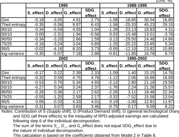
is an inequality index (for inequality level or its change) computed based on RPD-adjusted earnings.

It should be noted that summing the terms

S _

effect

,

D _

effect

, and

G _

effect

obtained above does not necessarily equal

SDG _

effect

. Alternatively, if we examine the effect of each factor sequentially by using the counterfactual distributions

f

(ln

W

)

_noS ,

noSD

W

f

(ln

)

(counterfactual distribution without supply shift and product demand shift), and

f

(ln

W

)

_noSDG, the sum of

S _

effect

,

D _

effect

,

G _

effect

is equal to

SDG _

effect

(i.e.

SDG _

effect

is exclusively decomposed into

S _

effect

,

D _

effect

,

G _

effect

). However, the magnitude of the effect of each factor changes with the order of decomposition in such a sequential decomposition. In order to avoid this problem, I have chosen to examine the effect of S, D, G individually, but not sequentially, in order to compare the importance of each of S_, D_, G_effect in an equal manner.

Step 7. Decomposing the inequality of RPD-adjusted earnings into SDG and other factors

First, following the regression-based decomposition method explained in Fields (2002), the inequality of each counterfactual RPD-adjusted earnings distribution with 1) no supply shift

(

f

(ln

W

)

_noS), 2) no product demand shift (

f

(ln

W

)

_noD), 3) no general technological change (

f

(ln

W

)

_noG), and 4) none of the three shifts (

f

(ln

W

)

_noSDG) is decomposed into

s

_j’s: the contribution of institutional and human capital factors (sex, minority status, Communist Party membership, experience, education, ownership, occupation, industry, employment status, province, and residual). Each

s

_j(the contribution of the j’th factor to the inequality level of a certain counterfactual earnings distribution) is computed from the following equation.

) (ln / ] ln , [ * ) ( * ) (ln / ] ln , cov[ ) (lnY a Z Y 2 Y a Z cor Z Y Y s_j = _{j j}

σ

= _j

σ

_{j j}

σ

where

ln

Y

is the logarithm of certain counterfactual earnings,

Z

_jis the j’th explanatory variable, and

a

_jis the estimated coefficient of the j’th factor obtained from the regression of

i

Y

ln

on J’s

Z

_j ,

σ

2 ,

σ

, and cor stand for variance, standard error, and correlation, respectively.

∑

+ = = 2 1 % 100 ) (ln J j j Y s , and

∑

+ = = 1 1 2 ) (ln ) (ln J j j Y R Y

s , where

R

2 stands for

R-squared, which represents the overall percentage explained by the explanatory variables (Fields 2002, Equations (8.a-d)).

Using the counterfactual earnings distributions,

Π

_j (the contribution of the j’th factor to the change in an inequality measure between time 1 and time 2) is also calculated as follows:

]

(.)

(.)

/[

]

(.)

*

(.)

*

[

(.))

(

I

s

_j,2

I

₂

s

_j,1

I

₁

I

₂

I

₁ j

=

−

−

Π

where

I

(.)

_t represents an inequality measure calculated at time t (t = 1 or 2), and

t j

s

_, represents the contribution of the j’th factor to the inequality level of lnY at time t. (Fields 2002, Equation (17.b)). I(.)₂ and

s

_j,2 are calculated based on the above counterfactual earnings distributions, while I(.)₁ and

s

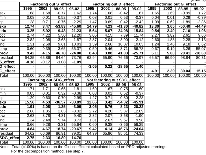
_j,1 are based on the actual earnings distributions.

The inequality (level or its change) of the actual RPD-adjusted earnings (=100%) is then decomposed into

S

_

effect

,

D

_

effect

, and

G

_

effect

(%) which are computed in step 6, and the contributions of other factors, each of which are calculated as:

(%)]

*

)

_

%

100

[(

−

S

effect

s

_j , when only

S

_

effect

is factored out.

(%)]

*

)

_

%

100

[(

−

D

effect

s

_j , when only

D

_

effect

is factored out.

(%)]

*

)

_

%

100

(%)]

*

)

_

%

100

[(

−

SDG

effect

s

_j , when

SDG

_

effect

is factored out.

For more details on the regression-based decomposition method, refer to Asuyama (2008) and Fields (2002).

3.2 Construction of skill groups and industry classification

Previous studies (i.e. Bound and Johnson, 1992; DiNardo, Fortin, & Lemieux, 1996; Liu, Park, & Zhao, 2007) constructed approximately 30 skill groups by dividing the entire sample into sex-education-experience groups. In my analysis on urban China, I have used region (whether coastal or inland region) instead of sex, and have constructed 30 region-education-experience skill groups.9 As mentioned in Asuyama (2008), labor market

segmentation by province exists in urban China. Institutional forces such as local government policy together with a different level of demand for labor due to a different pace of economic development may have created this segmentation by province. Since the model explained in this section assumes a competitive labor market, in order to alleviate the violation of the model, I have introduced a regional factor into the construction of skill groups by assuming that regional differences strongly affect the supply and demand (especially demand) of education-experience groups. Since my CHIP sample is too small to construct skill groups by province-education-experience, I have used two regional categories: coastal region and inland region. It is well known that the coastal region has achieved economic development more rapidly than the inland region. Thus, it is expected that demand for labor is higher in the coastal region than in the inland region. Following Kanbur and Zhang (2005) and other previous studies, Beijing, Liaoning, Jiangsu, and Guangdong are classified as the coastal region. The remaining provinces, Shanxi, Anhui, Henan, Hubei, Yunnan, and Gansu are classified as the inland region. It would be more desirable if I could also divide the region-education-experience group by sex. However, due to the small sample size, supply and demand differences in sex are not

9

I am deeply appreciative of Professor Fields, who suggested to me that I examine supply and demand differences between coastal and inland regions.

taken into account in this analysis. However, including region instead of sex seems more appropriate considering that labor market segmentation by province is much more significant than that by sex in urban China as seen in Table 1 and Table 2.

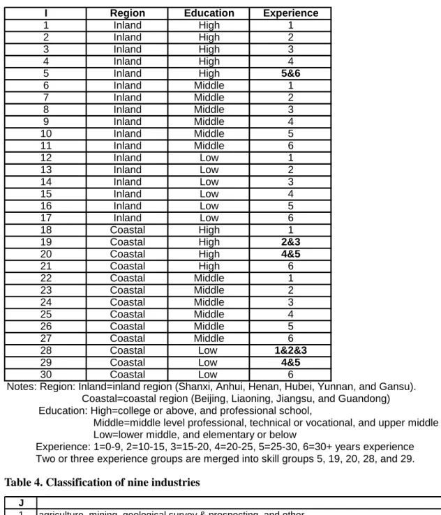
In this way, I have divided the entire sample into 30 region-education-experience skill groups and nine industries. There are two regions (coastal or inland), three education groups (High edu = college or above, and professional school, Middle edu = middle level professional, technical or vocational, and upper middle school, Low edu = lower middle school, and elementary school or below), and six experience groups (1 = 0-9, 2 = 10-15, 3 = 15-20, 4 = 20-25, 5 = 25-30, and 6 = 30+ years experience). Although all region-education-experience group combinations total 36 (2*3*6) groups, I have merged several experience groups into region-education groups in order to avoid zero observation in each cell ij. As a result, there are 30 skill groups. Classification of skill groups and industries is presented in Table 3 and Table 4, respectively.

When dividing observations in each skill group by nine industries, many cells contain a small number of observations. Although this can be a cause of error in the estimation procedure, a small number of skill groups and industries can also cause error. Nearly 30 skill groups are required in order to estimate each skill group’s earnings change due to the changes in SDG, since the number of observations used in the regression equation (1) equals the number of skill groups. A greater number of industry groups enables a more precise estimate of the relative demand shift between industries. Thus, 30 skill groups and nine industries are used in this analysis.

4. Results

4.1 Estimation of

Δ

ln

W

i,t,

SUP

i,t,

DEM

i,t, and

Δ

(ln

x

j

)

Table 5 displays the estimation result of

Δ

ln

W

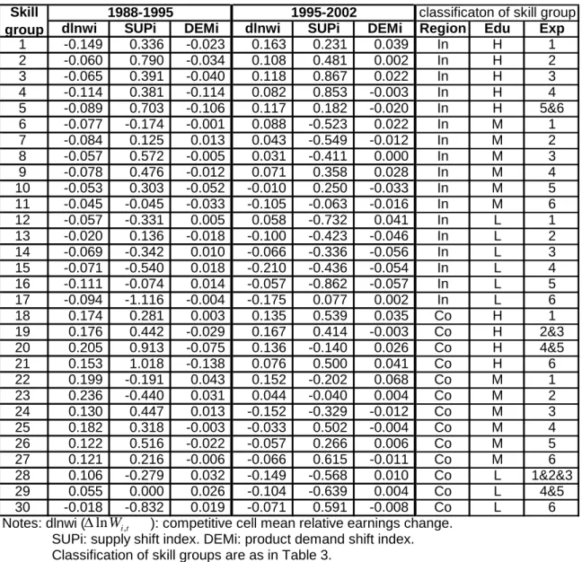
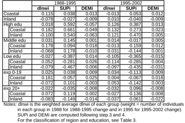
i,t(competitive cell mean relative

skill groups from both periods, 1988 to 1995 and 1995 to 2002. (The classification of the 30 skill groups are presented in Table 3.) In order to make the interpretation of Table 5 easier, Table 6 aggregates the results of Table 5 by two regions, three education groups, two experience groups, and the education and experience groups by two regions. As shown in Table 6, from 1988 to 1995, the estimated

Δ

ln

W

_i,t(see columns labeled dlnwi) is positive for the coastal region, the highly educated (college and above, and professional school) and the middle-level educated (middle level professional, technical or vocational, and upper middle school), and the less experienced (0-19 years experience). It is negative for the inland region, the low educated (lower middle school, and elementary school and below), and the more experienced. From 1995 to 2002,

Δ

ln

W

_i,tis positive for the inland region, the highly educated, the middle-level educated, and the less experienced. As seen in Asuyama (2008), earnings inequality between coastal and inland regions declined from 1995 to 2002, and the movement of

Δ

ln

W

_i,t by region reflects that trend.

With regard to

SUP

_i,tand

DEM

_i,t, both the relative supply and product demand increased for the workers in the coastal region (or relative supply and product demand decreased for the workers in the inland region) in both periods. There is almost no change in the size of the relative product demand shift for the two regions in both periods. However, the relative labor supply increase in the coastal region (or the relative labor supply decrease in inland region) became greater from 1995 to 2002. The relative product demand increased for the low educated and the middle-level educated, while it decreased for the highly educated from 1988 to 1995. In contrast, from 1995 to 2002, the relative product demand increased for the highly educated and the middle-level educated, and decreased for the low educated. The supply of the highly educated increased substantially, while that of the low educated decreased greatly during both periods. During both periods, the relative product demand increased for the less experienced group. The relative supply of the less experienced (0-19 years experience) when compared to the more experienced (20+ years experience), increased from 1988 to 1995, while it decreased from 1995 to 2002. The relative supply and product demand shifts were both larger in the

coastal region in the most educated and experienced groups.

As explained in step 4 in the previous section, in advance of estimating

DEM

_i,t,

)

(ln

x

_j

Δ

(relative product demand shift for industry j) must be estimated. Table 7 reports the estimation results of

Δ

(ln

x

_j

)

for both periods. For the period from 1988 to 1995, the relative product demand shift is positive and largest for industry 6 (real estate, public utilities, personal & consulting services, social services, and finance & insurance), followed by industry 5 (commerce & trade, restaurants & catering, materials supply, marketing, and warehousing), and industry 9 (government, Party organs, and social organizations). The coefficient for manufacturing (industry 2) is also positive but statistically insignificant. In contrast, the relative demand shifts for industries such as industry 1 (agriculture, mining and other), 3 (construction), 8 (education and scientific research), 7 (health, physical culture and social welfare), and 4 (transportation, communications, and post & telecommunications) are negative.

For the period from 1995 to 2002, the relative demand shift is positive and largest for industry 6 (real estate, public utilities, personal & consulting services, social services, and finance & insurance), followed by industry 1 (agriculture, mining and other), industry 4 (transportation, communications, and post & telecommunications), and industry 3 (construction). A negative relative demand shift is observed for industry 5 (commerce & trade, restaurants & catering, materials supply, marketing, and warehousing), industry 2 (manufacturing), and industry 9 (government, Party organs, and social organizations). The coefficients for industry 7 (health, physical culture and social welfare) and 8 (education and scientific research) are not statistically significant. In sum, a demand increase for some service industries and a demand decrease for manufacturing (only for the 1995-2002 period) are observed. As examined in the data description section of Asuyama (2008), the employment share of manufacturing declined dramatically from 41.1% to 25.2% between 1995 and 2002 in my CHIP sample. This is consistent with the statistics of total urban employment drawn from the China Labour Statistical Yearbook (CLSY). CLSY reports that the proportion of manufacturing in urban employment declined from 35.9% to 27.1% in the period 1995 to 2002. Although the relative demand

increase for industry 1 (agriculture, mining, and other) seems unexpected, the employment share of those mixed industries increased in my CHIP sample due to the share increase in mining and other industries. However, in the CLSY statistics, the proportion of industry 1 declined slightly from 11.7% to 11.1%.

4.2 Estimated cell mean earnings change due to the changes in SDG

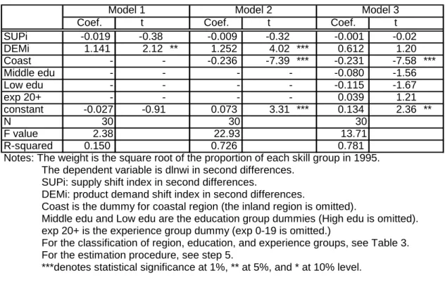
Table 8 presents the WLS regression results of

Δ

ln

W

_i,t on

SUP

_i,t and

DEM

_i,t. In Model 1, only

SUP

_i,t and

DEM

_i,tare included as explanatory variables. The pace of technological change

(

Δ

ln

b

_i,t2

−

Δ

ln

b

_i,t1

)

is assumed to be identical across all skill groups and

(

1

−

1

/

σ

)(

Δ

ln

b

_i,t2

−

Δ

ln

b

_i,t1

)

is treated as a constant term. The obtained coefficients are -0.019 for

SUP

_i,t and 1.141 for

DEM

_i,t with F-Statistics 2.4 (p-value: 0.11), although the estimated coefficient for

SUP

_i,t is not statistically significant.

Next, in order to check whether the initial assumption of an identical technological growth across all skill groups is appropriate, dummies for the region, education, and experience groups were added. Only the region dummy was added in Model 2, and region, education, and experience dummies were all added in Model 3. The results of Model 2 and Model 3 clearly show that only the coefficient for the region dummy is statistically significant and the addition of a region dummy greatly increases the goodness of fit of the model (i.e. the region factor explains the largest part of the competitive earnings change). Adding only a region dummy does not change the coefficients for

SUP

_i,t and

DEM

_i,tsignificantly. In Model 2, the coefficients for

SUP

_i,tand

DEM

_i,tare -0.009 and 1.252, respectively. Again, the coefficient for

SUP

_i,tis statistically insignificant.

The results from Model 1 and Model 2 suggest that: 1) supply shift across skill groups did not affect the earnings change in urban China at all, or if there were any effects their magnitude was very small, 2) in contrast, product demand shift did affect the earnings change in urban China from 1988 to 2002. Also, if we interpret our theoretical model literally, the result from Model 2 indicates that 1) earnings changes in skill groups were largely explained by

general technological change, 2) the pace of technological change was not identical, but differed across skill groups (i.e.

A

_i

=

A

₀

+

A

_1i ), and 3) the pace of technological change was greater in the inland region (What “general technological change” really stands for and the validity of the theoretical model will be examined in the discussion section below).

4.3 Contribution of SDG to earnings inequality

Since the explanatory power and the overall statistical significance of Model 2 is much better than Model 1, and the fact of the declining earnings inequality between the coastal and inland regions from 1995 to 2002 is consistent with the results of Model 2, I have used Model 2 to analyze the contribution of the supply shift, product demand shift, and general technological change to earnings inequality.10 Although the coefficients for

SUP

_i,t are not statistically significant, by using the coefficients obtained from Model 2 in Table 8, and following step 5, I have estimated the competitive cell mean relative earnings change due to 1) the supply shift (

−

(

1

/

σ

)

SUP

_i,t), 2) the product demand-shift (

(

1

/

σ

)

DEM

_i,t), and 3) the remaining factor, which represents general technological change (

(

1

−

1

/

σ

)

Δ

ln

b

_i,t). The estimated results are presented in Table 9. First, it is clear that the competitive cell mean relative earnings change for all groups can be largely explained by the remaining factor, representing general technological change. Second, the competitive cell mean earnings change due to the remaining factor is greater for the higher educated and the less experienced in both periods. It is greater for the coastal region in the period 1988 to 1995, but greater for the inland region in the period 1995 to 2002. Third, since the coefficient for

SUP

_i,tis very small, the magnitude of earnings change due to supply shift is almost always smaller than that due to product demand shift.

Next, I constructed four counterfactual earnings distributions,

f

(ln

W

)

_noS ,

noD

W

f

(ln

)

,

f

(ln

W

)

_noG, and

f

(ln

W

)

_noSDG by using the coefficients obtained from Model 2. Following step 6, the effects of 1) supply shift (

S

_

effect

), 2) product-demand shift

10

However, since the size of the coefficients for SUPi and DEMi are almost the same in Model 1 and Model 2, using Model 1 does not significantly change the result of supply and product demand shift effects obtained.