トップ - アジア経済研究所学術研究リポジトリ ARRIDE

(1)

Allocation efficiency in China's state-owned,

private, and foreign sector firms

著者

Hashiguchi Yoshihiro

権利

Copyrights 2020 by author(s)

journal or

publication title

IDE Discussion Paper

volume

778 year

2020-03

(2)

INSTITUTE OF DEVELOPING ECONOMIES

IDE Discussion Papers are preliminary materials circulated to stimulate discussions and critical comments

Keywords: Misallocation, Firm-level productivity, Structural estimation, China JEL classification: D24, O47

* Research Fellow, Economic Modelling Studies Group, Development Studies Center, IDE ([email protected])

IDE DISCUSSION PAPER No. 778

Allocation Efficiency in China's

State-owned, Private, and Foreign

Sector Firms

Yoshihiro HASHIGUCHI*

March 2020

Abstract

Despite the fact many scholars have shown an interest in China's allocation efficiency, few studies have examined quantitative analysis of allocation efficiency within and between the state-owned and private sectors. To address this issue, this paper develops a quantitative measure of allocation efficiency, which is an extension of the dynamic Olley-Pakes productivity decomposition proposed by Melitz and Polanec (2015). The extended measure enables the simultaneous capture of the degree of misallocation within a group and between groups and parallel to capturing the contribution of entering and exiting firms to aggregate productivity growth. Using China's manufacturing firm-level data from 2003 to 2007, the author examine the efficiency of resource allocation within and between three ownership sectors (state-owned, domestic private, and foreign sectors). It is found that the between allocation efficiency tends to improve in industries wherein market shares move from the less-productive state sector to the more-productive private sector.

(3)

The Institute of Developing Economies (IDE) is a semigovernmental, nonpartisan, nonprofit research institute, founded in 1958. The Institute merged with the Japan External Trade Organization (JETRO) on July 1, 1998. The Institute conducts basic and comprehensive studies on economic and related affairs in all developing countries and regions, including Asia, the Middle East, Africa, Latin America, Oceania, and Eastern Europe.

The views expressed in this publication are those of the author(s). Publication does not imply endorsement by the Institute of Developing Economies of any of the views expressed within.

INSTITUTE OF DEVELOPING ECONOMIES (IDE), JETRO

3-2-2, WAKABA,MIHAMA-KU,CHIBA-SHI

CHIBA 261-8545, JAPAN

No part of this publication may be reproduced without the prior permission of the author(s).

(4)

Allocation E

ﬃciency in China’s State-owned, Private,

and Foreign Sector Firms

∗

Yoshihiro HASHIGUCHI

†

Institute of Developing Economies

March 2020

Abstract

Despite the fact many scholars have shown an interest in China’s allocation eﬃciency,

few studies have examined quantitative analysis of allocation eﬃciency within and between

the state-owned and private sectors. To address this issue, this paper develops a

quantita-tive measure of allocation eﬃciency, which is an extension of the dynamic Olley-Pakes

productivity decomposition proposed by Melitz and Polanec (2015). The extended mea-sure enables the simultaneous capture of the degree of misallocation within a group and between groups and parallel to capturing the contribution of entering and exiting firms to aggregate productivity growth. Using China’s manufacturing firm-level data from 2003 to 2007, the author examine the eﬃciency of resource allocation within and between three ownership sectors (state-owned, domestic private, and foreign sectors). It is found that the

between allocation eﬃciency tends to improve in industries wherein market shares move

from the less-productive state sector to the more-productive private sector.

Keywords: Misallocation, Firm-level productivity, Structural estimation, China

JEL classification: D24, O47

∗_{I would like to thank participants at the Fudan University Workshop 2014, the OECD Mini-Conference 2014,}

and the Institute of Developing Economies Workshop for their constructive comments. All remaining errors are my own.

†_{Address: 3-2-2 Wakaba, Mihama-ku, Chiba-shi, Chiba 261-8545 Japan.}

(5)

1 Introduction

Recent studies argued that the allocation of production resources among firms or sectors is a key driver behind the growth of aggregate total factor productivity (TFP) (Restuccia and Roger-son, 2008; Hsieh and Klenow, 2009; Bartelsman et al., 2013; Collard-Wexler and De Loecker, 2015). The shift in production resources from less productive to more productive units yields

an increase in aggregate TFP, and resource allocation eﬃciency can be crucial to explaining

countries’ aggregate TFP. A well-functioning market economy has a function to allocate more production resources to more productive businesses. Because developing economies are

gen-erally found to have lower allocation eﬃciency than developed economies, improving resource

allocation is expected to increase their aggregate TFP and GDP per capita.

In this paper, the author investigates the allocation of production resources in China’s

man-ufacturing sector. Several scholars have argued the degree of allocation eﬃciency in China. For

example, Hsieh and Klenow (2009) used manufacturing firm-level data from 1998 to 2005 to measure the degree of misallocation and found that misallocation within an industry tended to decline over time. Chen, et al. (2011) used industry-level data from 1980 to 2008 and found that factor reallocation played a substantial role in increasing aggregate productivity from 1980

to 2000; however, after 2001, they found that allocation eﬃciency worsened and contributed to

decreasing productivity growth. Brandt, et al. (2013) also used industry-level data by province from 1985 to 2007 and found that misallocation within provinces declined between 1985 and 1997 but increased in the last 10 years.

Although many researchers have maintained continuous interests in the allocation eﬃciency

in China, little study has been done to actually explore resource allocation between ownership sectors. Since the 2000s, one debate has been over the state sector’s advantageous access to capital resources compared with the private sector, a phenomenon called Guojin Mintui (i.e., the state advances, the private sector retreats). Such a favorable environment for the state sector may impede the growth of the private sector, causing resource allocation to deteriorate. Has

China’s resource allocation between the state and private sector been working eﬃciently? There

are no definitive answers to this questions.

To address this issue, the author develops a quantitative measure of allocation eﬃciency,

which is an extension of the dynamic Olley-Pakes productivity decomposition proposed by

Melitz and Polanec (2015).1) The covariance measure was originally proposed by Olley and

Pakes (1996), Melitz and Polanec (2015) extended it to capture the contributions of entering and exiting firms, calling it the dynamic Olley-Pakes (OP) productivity decomposition. However,

the dynamic and non-dynamic (i.e., original) OP decomposition do not capture allocation e

ﬃ-ciency between groups (e.g., ownership groups); they only capture allocation eﬃciency within

a group. This paper attempts to extend the dynamic OP decomposition to a multi-group version

to simultaneously capture the degree of allocation eﬃciency within a group and between groups

and parallel to capturing the contribution of entering and exiting firms. Using this extended

de-composition, the author examines the allocation eﬃciency within and between the state-owned,

1)_{There are two types of empirical measures of allocation e}_{ﬃciency: (1) the gap beween marginal product and}

the unit cost of input (Hsieh and Klenow, 2009; Petrin and Levinsohn, 2012) and (2) the covariance between a firm’s market share and productivity (Olley and Pakes, 1996; Collard-Wexler and De Loecker, 2013; Melitz and Polanec, 2015). This paper attempts to extend the latter measure of allocation eﬃciency.

(6)

domestic private, and foreign sectors.

The data used for the quantitative analysis is based on China’s manufacturing firm-level data from 2003 to 2007. The empirical analysis has two steps. First, firm-level productivity is estimated using a structural estimation method proposed by Gandhi, et al. (2016). Second, the

productivity decomposition method is exploited to quantify the eﬀect of misallocation on

aggre-gate manufacturing productivity. As a result, allocation eﬃciency between the three ownership

sectors (state-owned, domestic private, and foreign sectors) tends to improve in industries in which the market share moves from a less-productive state-owned sector to a more productive

private sector. However, this eﬃciency tends to worsen in industries in which 1) the state-owned

sector’s TFP increases on relative basis despite decreases in its market share or 2) the private sector’s TFP does not grow compared with other sectors despite increases in its market share.

The remainder of this paper is structured as follows. Section 2 describes the measure of

allocation eﬃciency used in this study. Section 3 describes the TFP estimation procedure and

the data sources, Section 4 reports the allocation eﬃciency in China, and Section 5 concludes.

2 Measure of Allocation E

ﬃciency

The measure of allocation eﬃciency used in this paper is based on a productivity

decomposi-tion method originally developed by Olley and Pakes (OP; 1996) and extended by Melitz and Polanec (MP; 2015) to a dynamic version. Sections 2.1 and 2.2 review the OP and MP methods, and Section 2.3 describes the extended version of their methods. Section 4 reports the empirical

results of allocation eﬃciency between ownership groups.

2.1 Olley-Pakes Decomposition

Let us consider aggregate productivity (Φt), which is defined as the weighted average of

firm-level productivity: Φt =

∑

i∈Ωt sitϕit, whereΩtis the set of firms at time t,ϕitis the firm-level log

TFP, and sitis firm i’s share of output at time t. Olley and Pakes (1996) showed that aggregate

productivity can be decomposed into the following two parts: Φt = ∑ i∈Ωt sitϕit = 1 Nt ∑ i∈Ωt ϕit+ ∑ i∈Ωt   sit− 1 Nt ∑ ι∈Ωt s_ιt      ϕit− 1 Nt ∑ ι∈Ωt ϕιt    = µt+ covt (1)

where µt represents the unweighted mean productivity and covt is proportional to the

covari-ance between market shares and productivity. covt represents the magnitude of allocation e

ﬃ-ciency because it increases as more-productive firms have higher market shares, and conversely, it decreases as less productive firms have higher market shares. Olley and Pakes (1996) used plant-level panel data on the U.S. telecommunications equipment industry from 1974 to 1987 to estimate plant-level productivity for the industry and then exploited it to calculate OP

decom-position. They found that the unweighted mean productivity (µt) did not change much since

1975, but the covariance term increased from 0.01 in 1974 to 0.32 in 1987. They concluded that a factor reallocation occurred from less-productive to more-productive plants.

(7)

2.2 Dynamic Olley-Pakes Decomposition

Melitz and Polanec (2015) extended the OP decomposition to capture the contribution of en-tering and exiting firms in aggregate productivity, which is called the dynamic Olley-Pakes

productivity decomposition. They showed that the diﬀerence in the aggregate log TFP at times

1 and 2 (∆Φ = Φ2 − Φ1) can be decomposed into the following parts: (1) unweighted TFP

of firms surviving during the period, (2) the OP’s covariance term calculated using surviving firms’ log TFP and market shares, and (3) the contribution of entering and exiting firms during the period.

The dynamic Olley-Pakes (DOP) decomposition is derived as follows. First, the aggregate

log TFP at time 1 (Φ1) is decomposed into surviving firms’ log TFP and exiting firms’ log TFP

at time 1: Φ1 = ∑ i∈ΩS si1ϕi1+ ∑ i∈ΩX si1ϕi1 = ΦS 1 + s X 1 ( ΦX 1 − Φ S 1 ) , (2)

whereΩS andΩX denote the sets of surviving and exiting firms during the period andΦS₁ and

ΦX

1 are the aggregate log TFPs at time 1 for surviving and exiting firms, respectively:

ΦS 1 = ∑ i∈ΩS si1 ∑ ι∈ΩS sι1ϕ i1, ΦX1 = ∑ i∈ΩX si1 ∑ ι∈ΩX sι1ϕ i1, sX1 = ∑ i∈ΩX si1.

Similarly, the aggregate log TFP at time 2 is decomposed into surviving firms’ log TFP at time 2 and entering firms’ log TFP at time 2:

Φ2 = ∑ i∈ΩS si2ϕi2+ ∑ i∈ΩE si2ϕi2 = ΦS 2 + s E 2 ( ΦE 2 − Φ S 2 ) , (3)

whereΩE _{denotes the set of entering firms during the period and}ΦS

2 andΦ E

2 are the aggregate

log TFPs at time 2 for surviving firms and entering firms, respectively: ΦS 2 = ∑ i∈ΩS si2 ∑ ι∈ΩS sι2 ϕi2, ΦE2 = ∑ i∈ΩE si2 ∑ ι∈ΩE sι2 ϕi2, sE2 = ∑ i∈ΩE si2.

Applying the OP decomposition toΦS

t (t= 1, 2) yields: ΦS t = 1 NS ∑ i∈ΩS ϕit+ ∑ i∈ΩS   ∑ sit ι∈ΩS sιt − 1 NS ∑ i∈ΩS sit ∑ ι∈ΩS sιt      ϕit− 1 NS ∑ i∈ΩS ϕit    = µS t + cov S t, (4)

where NS is the number of firms surviving during the period,µSt is the unweighted mean

pro-ductivity of surviving firms, and covS

(8)

surviving firms. Substituting Equation (4) in Equations (2) and (3) and taking the diﬀerence of

the aggregate log TFP (∆Φ = Φ2− Φ1) results in the DOP decomposition as follows:

∆Φ = ∆µS _{+ ∆cov}S _{+ s}E 2(Φ E 2 − Φ S 2)+ s X 1(Φ S 1 − Φ X 1)

= ∆µS _{+ ∆cov}S _{+ ent + ext ,} (5)

where ∆µS = µS 2 − µ S 1, ∆cov S = covS 2 − cov S 1, ent = s E 2(Φ E 2 − Φ S 2), and ext = s X 1(Φ S 1 − Φ X 1).

The first term on right-hand side is the change in the unweighted average log TFP for surviving firms. The second term is the change in the covariance, which indicates the change in the

magnitude of allocation eﬃciency among surviving firms. The contributions of entering and

exiting firms appear in ent and ext, respectively, both of which are evaluated in comparison with the productivity of surviving firms as follows:

ent ⋚ 0 when ΦE₂ ⋚ ΦS₂, ext ⋚ 0 when ΦS₁ ⋚ ΦX₁.

Thus, the DOP decomposition method allows us to identify the contributions of entering and exiting firms.

Melitz and Polanec (2015) used firm-level panel data from the Slovenian manufacturing sector from 1995 to 2000 to estimate the parameters of a production function for the industry and then calculated the DOP decomposition using the estimated log TFP and the log of labor

productivity. They found that the aggregate log TFP change (∆Φ) from 1995 to 2000 is 0.4013

and is decomposed into the unweighted mean productivity for surviving firms (∆µS = 0.2758),

the covariance term change (∆covS = 0.0955), and the contributions of entering and exiting

firms (ent = 0.0021, ext = 0.0279). Their results indicate that the improvement in allocation

eﬃciency added 10 percentage points to aggregate TFP growth during the five years.

2.3 Augmented Dynamic OP (ADOP) Decomposition

The OP and DOP decompositions allow us to quantify the degree of allocation eﬃciency within

a group (e.g., an industrial sector). However, these quantifications can be augmented to a

multi-group version to simultaneously capture the degree of allocation eﬃciency within a group and

between groups. This section shows the augmented version of the DOP decomposition.

Let us consider that the number of groups is J and aggregate log TFP at time 1 is represented as: Φ1= ∑J j=1wj1 ∑ i∈Ωj1 si1 wj1ϕ i1 = ∑J_j₌₁wj1µ˜j1,

where Ωj1 is the set of firms in group j at time 1, wj1 is group j’s output share at time 1,

and ˜µj1 =

∑

(9)

decomposition to the above equation yields: Φ1= 1 J ∑J j=1µ˜j1+ ∑J j=1 ( wjt− 1 J ∑J κ=1wκ1 ) ( ˜ µj1− 1 J ∑J κ=1µ˜κ1 ) = 1 J ∑J j=1µ˜j1+ ˜cov1, (6)

where cov˜ t represents the magnitude of inter-group allocation eﬃciency. This paper defines

the first and second terms as “within-eﬀect” and “between-eﬀect,” respectively. The weight

ai j1 = si1/wj1 can be written as ∑ i∈Ωj1 ai j1 = ∑ i∈ΩS j ai j1+ ∑ i∈ΩX j ai j1 = aS j1+ a X j1 = 1. whereΩS j andΩ X

j denote the sets of surviving and exiting firms for group j, respectively. They

can be decomposed into the weighted average log TFP of surviving firms and the contribution of exiting firms: ˜ µj1 = ∑ i∈ΩS j ai j1 aS_j1ϕi1+ a X j1   _i∑_∈ΩX j ai j1 aX_j1ϕi1− ∑ i∈ΩS j ai j1 aS_j1ϕi1    = ΦS j1+ a X j1 ( ΦX j1− Φ S j1 ) = ΦS j1− extj, (7) whereΦS j1andΦ X

j1denote the weighted average log TFP of surviving and exiting firms for group

j, respectively, and extj = aX_j1

( ΦS j1− Φ X j1 )

represents the contribution of exiting firms to group

j’s aggregate productivity ˜µj1. By exploiting the OP decomposition method, the first term of

Equation (7) can be decomposed as:

ΦS j1 = 1 NS j1 ∑ i∈ΩS j ϕi1+ ∑ i∈ΩS j   ai j1 aS j1 − 1 NS j1 ∑ ι∈ΩS j a_{ι j1} aS j1      ϕi1− 1 NS j1 ∑ ι∈ΩS j ϕι1    = µS j1+ cov S j1, (8) whereµS

j1 is the simple average log TFP of surviving firms at time 1 and cov

S

j1 is the degree of

allocation eﬃciency within group j at time 1. Substituting Equations (8) and (7) in Equation

(6) yields the following decomposition:

Φ1= 1 J ∑J j=1 ( µS j1+ cov S j1− extj ) | {z } Within eﬀect + |{z}cov˜ 1 Between eﬀect . (9)

(10)

Similarly, the aggregate log TFP at time 2 can be decomposed as follows: Φ2 = 1 J ∑J j=1µ˜j2+ ˜cov2 = 1 J ∑J j=1 ( ΦS j2+ a E j2 ( ΦE j2− Φ S j2 )) + ˜cov2 = 1 J ∑J j=1 ( µS j2+ cov S j2+ entj ) | {z } Within eﬀect + |{z}cov˜ 2 Between eﬀect , (10) where entj = aE_j2 ( ΦE j2− Φ S j2 )

indicates the contribution of entering firms to aggregate produc-tivity ˜µj2.

Finally, taking the diﬀerence between Φ1 and Φ2, the augmented dynamic OP (ADOP)

decomposition is obtained: ∆Φ = 1 J ∑J j=1 ( ∆µS j + ∆cov S j + entj+ extj ) | {z } Within eﬀect + ∆ ˜_|{z}cov Between eﬀect (11)

where∆covS_j represents the changes in allocation eﬃciency among surviving firms within group

j and∆ ˜cov represents the changes in allocation eﬃciency between groups. When J = 1, Equa-tion (10) reduces to the original dynamic OP decomposiEqua-tion.

In this paper, Equation (11) is used to decompose China’s aggregate productivity and

in-vestigate the magnitude of allocation eﬃciency within and between ownership sectors. The

empirical results are described in Section 4. Before reporting the results, the next section ex-plains how to measure firm-level productivity (ϕit).

3 Production Function Estimation and Data Description

3.1 Production Function Estimation

Having clarified the measure of allocation eﬃciency in the previous section, showing the

mea-sure of firm-level productivity is required. This paper employs the nonparametric identification strategy proposed by Gandhi, et al. (GNR; 2016) to measure China’s firm-level productivity. This method is built on the recent literature on production function estimation, such as Olley and Pakes (1996), Levinsohn and Petrin (LP; 2003), and Ackerberg, et al. (ACF; 2006). The Appendix A contains GNR’s estimation methodology used in this study.

3.2 Data Description

The data used to estimate the production function are based on unbalanced firm-level panel data on China’s manufacturing industry from 2003 to 2007, which are obtained from the annual survey of industrial enterprises conducted by the National Bureau of Statistics. The survey covers firms with sales higher than 5 million RMB in the mining, manufacturing, and public utilities industries, and the original database consists of 336,768 industry firms for 2007, which

(11)

is the same number as that reported in the China Statistical Yearbook published in 2008 (p.

485). Firm IDs contained in the database are used to construct a panel of observations.2)

The production function variables are constructed as follows: Yitis the total gross output, Kit

is the total fixed assets, Litis the number of employees, and Mitis the total intermediate inputs.

The deflators for Yit and Mit are based on the output and input deflators provided by Brandt, et

al. (2012).3)_{The deflator for total fixed assets is constructed as follows.}

(1) Firm-level total fixed-asset data at current prices are gathered by province. The province-level data are denoted by ˜Kpt, where p denotes a province.

(2) The provincial nominal investment is calculated as ˜Iit = ˜Kpt − (1 − δ) ˜Kp,t−1. Following

Brandt et al. (2012), the depreciation rateδ is set at 0.09.

(3) ˜Iit is deflated by a province-level investment deflator, which is obtained from the China

Statistical Yearbook. Using the deflated investment (Ipt), provincial deflated fixed assets

are calculated as Kpt = (1 − δ)Kp,t−1+ Ipt, where Kp0 = ˜Kp0.

(4) The deflator for total fixed assets by province can be calculated using ˜Kpt and Kpt.

The following firms are removed as outliers from the database: 1) firms with a non-positive value for Yit, Kit, Lit, or Mit; 2) firms whose Yit/Litor Kit/Litin t is more than 1000 times or less

than 0.001 the value in t − 1; or 3) firms in Tobacco (industrial codes 161, 162, and 169) and

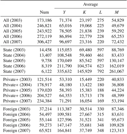
nuclear-related industries (253 and 424). Table 1 shows the number of firms. Manufacturing firm-level data without outliers are used for the estimation.

[– Table 1 –]

Table 2 reports summary statistics of the panel data by ownership sector. “State” denotes state-owned firms, including state-owned enterprises and solely state-funded corporations.

“Pri-vate+” denotes domestic and non-state-owned firms, including collective-owned firms (and

other hybrids) and privately funded enterprises. “Foreign” denotes firms with funds from Hong Kong, Macao, and Taiwan and those that are purely foreign-funded enterprises. The State sector shows the smallest number of firms and a sharp decrease of 57% from 2003 to 2007, whereas

the number of private and foreign firms increased during the four years. The Private+ sector has

the largest number of firms, accounting for 76% of the total in 2007. However, its output per firm is nearly five times smaller than that of state-owned firms in 2007, indicating that most pri-vate firms operate as small entities compared with state and foreign firms. Note that the number of firms in 2004 increases 1.4 times compared to the previous year. Because Chinese economic census was conducted in 2004, the sample coverage has been probably expanded since 2004.

[– Table 2 –]

2)_{However, this IDs are often missing or changes over time. Hence, this paper creates a new series of firm IDs}

by using firm attributes, such as original firm IDs, firm names, and phone numbers. Firm-matching is conducted by R. The matching algorithm is described in Appendix B.

(12)

3.3 Estimates of Output Elasticities

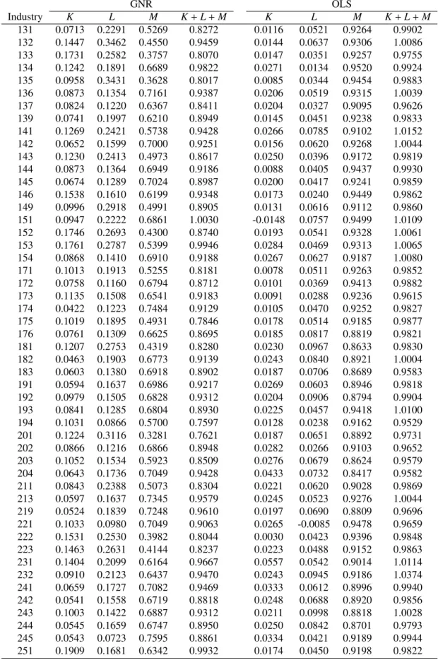
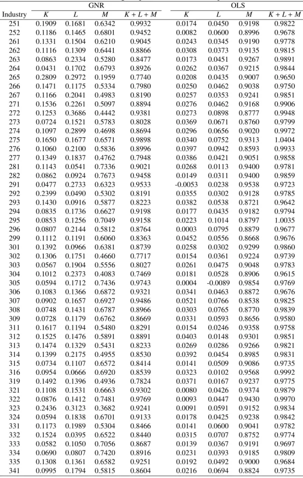
The production function is separately estimated by industry using a three-digit industrial code.4)

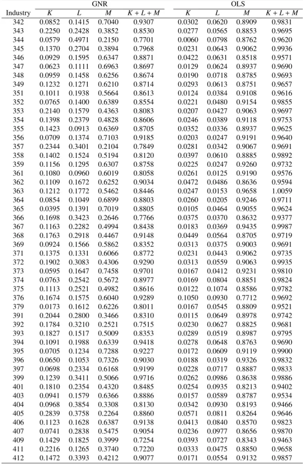
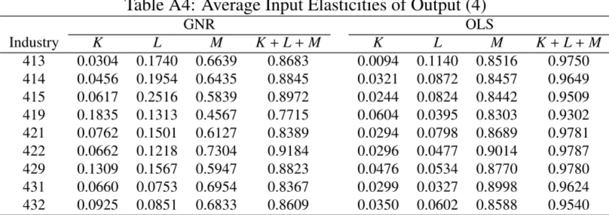
Appendix Tables A1–A4 report the estimates of the average output elasticities for each input and the sum of the elasticities for capital, labor, and intermediate inputs. The estimates of

GNR’s method are found to show lower average elasticities of intermediate inputs (ηM) than

the OLS estimates in every industry. The diﬀerence between the GNR and OLS estimates of

ηM is 0.32 on average, and the OLS estimates are approximately 1.55 times higher on average

than the GNR estimates. These results are clearly expected and consistent with the estimation results in GNR (2016). The failure to control the endogenous bias from the correlation between

flexible variables and unobservable productivity (ωit) is known to lead to overestimates of the

coeﬃcients on flexible variables because positive productivity shocks are likely to increase the

use of flexible inputs. The average elasticities of capital and labor as estimated by OLS are lower than the estimates based on the GNR method, which is also consistent with the empirical results in GNR (2016).

China’s intermediate input elasticities shown in Appendix Tables A1–A4 are similar to Colombia’s and Chile’s as estimated by GNR (2016). The data used in GNR (2016) are based on five three-digit manufacturing industries (Food Products, Textiles, Apparel, Wood Products, Fabricated Metal Products), and their estimates of input elasticities for these industries are 0.54 for Colombia, and 0.55 for Chile, respectively. This paper’s average elasticity for the nearly corresponding industries (131, 171, 181, 203, and 341) is 0.53, which is slightly smaller than the estimates of Colombia and Chile.

4 Allocation E

ﬃciency

This section presents the results of the augmented dynamic OP (ADOP) decomposition us-ing China’s manufacturus-ing firm-level productivity. These methods enable us to simultaneously

quantify allocation eﬃciency within and between three ownership groups ( j ∈ {State (S ),

Pri-vate+ (P), and Foreign (F) sectors} (J = 3)). Because the three-digit industrial classification is

relatively narrow, several industries have few or no firms in any of the three ownership sectors. To focus on the industries in which the three ownership sectors coexist, this analysis is con-ducted on the three-digit industrial sectors with more than 50 firms for each ownership sector.

As a result, 75 industrial sectors are used for the analysis.5)_{The ADOP decomposition equation}

for sector i is written as

∆Φ(i) = 1 3 ∑ j∈{S,P,F} [ ∆µS j(i)+ ∆cov S

j(i)+ entj(i)+ extj(i)

]

+ ∆ ˜cov(i).

Note that i denotes a three-digit industrial sector and the ADOP decomposition applies sepa-rately for each i= 1, 2, . . . , 75.

4)_{Industries 212, 214, 233, 402, and 423 are included in 211, 219, 232, 409, and 429, respectively. The}

estima-tion is implemented using R version 3.3.1 (R Development Core Team, 2009).

5)_{This sample selection may cause us to select industrial sectors where the state-owned firms are likely to survive}

in the market. It is necessary to keep in mind that there may exist the inequality of competitive conditions between the state and non-state sectors in such sectors.

(13)

4.1 Allocation E

ﬃciency between Ownership Groups

[– Figure 1 –]

Figure 1 demonstrates the ADOP decomposition of the aggregate TFP growth from 2003 to

2007. The main driver of the aggregate TFP growth is∆covS

j(i), changes in the simple average

log TFP of surviving firms. The contribution of the within and between allocation eﬃciency

∆covS

j(i) and∆ ˜cov(i) varies across sectors, and the median of these contribution is much smaller

than those of∆covS_j(i). This indicates that resource reallocation does not contribute significantly to increasing the aggregate productivity growth.

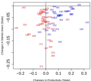
[– Figure 2 –]

Figure 2 presents the allocation eﬃciency between three ownership groups (∆ ˜cov(i)) during

2003–2007. This figure exhibits the plots of aggregate productivity changes ∆Φ(i) and the

changes in allocation eﬃciency between the three ownership groups, ∆ ˜cov(i). Although the

average of ∆ ˜cov(i) is almost zero, it varies among industries, ranging from −0.167 to 0.109.

In all, 42 industrial sectors are plotted in the positive area of the vertical axis (∆ ˜cov(i) > 0), indicating that these industries tend to improve resource allocation among the three ownership groups.

[– Figure 3 –]

To investigate the source of the variation in∆ ˜cov(i), it is rewritten as follows:

∆ ˜cov(i)= ∑

j∈{S,P,F}

[

xj2(i) yj2(i)− xj1(i) yj1(i)

]

= ∑

j∈{S,P,F}

[

yj2(i)∆xj2(i)+ xj1(i)∆yj2(i)

] (12)

where xjt(i)= wjt(i)− 1/J

∑

jwjt(i) and yjt(i)= ˜µjt(i)− 1/J

∑

jµ˜jt(i) for t = 1, 2. For industry i

and ownership sector j,∆xjt(i) is changes in market share and∆yjt(i) is changes in the centered

aggregate productivity during 2003–2007. The relationship among the three variables (∆ ˜cov,

∆xjt, and∆yjt) is plotted in Panels (A)–(C) of Figure 3 by ownership, where the horizontal axis

is∆xjt, and the vertical axis is∆yjt. The red-colored plots denote industries with positive∆ ˜cov

values in Figure 2, whereas the blue-colored plots denote industries with negative∆ ˜cov values.6) As shown in Panel (A), the State sector’s market shares decreased in most industrial sectors, and red plots in Panel (A) are primarily distributed in the third quadrant. This result indicates

that resource allocation between ownership groups (∆ ˜cov) tends to improve in industries in

which the State sector’s market share and productivity both decrease. In contrast, the blue plots 6)_{Note that the first and third quadrants in Panels (A)–(C) indicate the positive relationship between the changes}

in market share and productivity. However, this positive relationship does not necessarily produce positive∆ ˜cov values. As is clear from Equation (12),∆ ˜cov does not necessarily become positive even if the sign of∆xj2is the

(14)

in Panel (A) are primarily distributed in the fourth quadrant, indicating that the resource allo-cation between ownership groups are likely to worsen in industries in which the State sector’s market share decreases but productivity increases.

Panel (B) shows the relationship between the changes in the Private+ sector’s market share

and productivity. Contrary to Panel (A), the red and blue plots are primarily distributed in the first and second quadrants, respectively, indicating that the resource allocation between

ownership groups tends to improve in industries in which the Private+ sector’s market share

and productivity both increase and worsen in industries in which the Private+ sector’s market

share increases but productivity decreases. In contrast, the Foreign sector (Panel (C)) does not show a clear relationship between red and blue plots.

In summary, the allocation eﬃciency between ownership sectors tends to improve in

in-dustries in which the market share moves from the less-productive State sector to the

more-productive Private+ sector. In contrast, the allocation eﬃciency tends to worsen in industries

in which 1) the State sector’s productivity relatively increases despite a decrease in its market

share or 2) the Private+ sector’s productivity does not grow compared with the other sectors

despite an increase in its market share.

4.2 Within-E

ﬀects for Each Ownership Group

[– Figure 4 –]

Figure 4 reports the histograms of the within-eﬀects. The vertical axis defines the number

of three-digit industrial sectors (i = 1, 2, . . . , 75). Panels (A), (B) and (C) show allocation

eﬃciency ∆covS

j(i), entry eﬀects entj(i), and exit eﬀects extj(i) within a group j ∈ {S, P, F},

respectively.7)

Panel (A) shows that the medians of these histograms is−0.006 (State), 0.02 (Private+),

and 0.009 (Foreign), and that the shares of the number of sectors with∆covS_j(i)> 0 are 46.1%,

64.5%, and 54.0%, respectively. Although the values of ∆covS

j(i) are distributed broadly for

each group, the Private+ group tends to improve its allocation eﬃciency among firms during

2003–2007. The entry eﬀect in Panel (B) shows that the medians for each group are −0.003

(State), −0.018 (Private+), and −0.011 (Foreign), and the shares of the number of sectors with

entj(i) > 0 are 46.1%, 31.6%, and 40.8%, respectively. This result indicates that new entry

firms in all groups during 2003–2007 have, on average, lower productivity than existing firms

for each group.] Consequently, they have a negative eﬀect on aggregate productivity growth.

In particular, new entry firms in the Private+ sector tend to show relatively low productivity

compared to the other sectors. Furthermore, the exit eﬀect of the Private+ group shown in Panel

(C) is also small. The medians are 0.039 (State), 0.0061 (Private+), and 0.0095 (Foreign), and

the shares of the number of sectors with extj(i)> 0 are 80.3%, 56.6%, and 64.5%, respectively,

implying that relatively nonproductive firms in the Private+ group are not likely to exit the

market.

7)_{Appendix Figures A1–A4 demonstrate the bar-plots of the decomposition into the ownership sectors by 3-digit}

(15)

In summary, the Private+ sector tends to have more industrial sectors improving allocation

eﬃciency among firms, compared with State and Foreign sectors. However, the entry and exit

eﬀects for Private+ are very weak. In particular, the entry eﬀect has negative values for many

industrial sectors, indicating that new firms in the Private+ sector tend to be less productive than

existing firms and drive down aggregate productivity growth.

5 Conclusions

Despite the fact many scholars have shown an interest in China’s allocation eﬃciency, few

studies have examined quantitative analysis of allocation eﬃciency within and between the

state-owned and private sectors. The author addresses this issue, using China’s manufacturing

firm-level data and a new measure of allocation eﬃciency that is an extension of the productivity

decomposition methods proposed by Olley and Pakes (1996) and Melitz and Polanec (2015). This new measure enables us to simultaneously capture the degree of misallocation within a group and between groups, and parallel to capturing the contribution of entering and exiting firms to aggregate TFP growth. Because the methods used by Olley and Pakes (1996) and

Melitz and Polanec (2015) cannot capture the degree of allocation eﬃciency between groups,

this new measure can be considered a group-wise extension of their methods.

It is found that misallocation between three ownership groups declined in 42 of the 75 three-digit industrial sectors, indicating that these industries improved resource allocation among the three ownership groups. Furthermore, misallocation tended to decline in industries wherein

market shares move from the less-productive State sector to the more-productive Private+

sec-tor. In contrast, misallocation tended to worsen in industries in which 1) the State sector’s

productivity relatively increases despite decreases in its market share or 2) the Private+

sec-tor’s productivity does not grow compared with that of the other sectors despite increases in its market share.

These empirical results lead us to conclude that resource allocation between State, Private+,

and Foreign sectors tends to improve by allocating production resources to more productive private firms from less productive state-owned firms. In other words, industries in which less

productive state-owned firms have greater market share are likely to be lower allocation e

ﬃ-ciency. What is behind the behavior of allocation eﬃciency in China? According to previous

studies, financial frictions are believed to be an important source of misallocation (Caggese and Cu˜nat, 2013; Midrigan and Xu, 2014). The main source of misallocation between ownership sectors could be attributed to unequal access to factor resources, such as capital from bank loans, subsidies, and land, between state-owned and non-state owned firms. A favorable environment for the state sector or a phenomenon “Guojin Mintui” (i.e., the state advances, the private sector retreats) may impede the growth of the private sector, causing resource allocation to deteriorate. Although identifying the source of misallocation is challenging, reexamining the equity of com-petitive conditions among firms in the financial market in terms of optimal resource allocation is crucially important.

(16)

References

Ackerberg, D. A., K. Caves, and G. Frazer. (2006) “Structural identification of production function.” Unpublished Manuscript, UCLA Economics Department.

Bartelsman, E., J. Haltiwanger, and S. Scarpetta. (2013) “Cross-country diﬀerences in

produc-tivity: the role of allocation and selection.” American Economic Review, 103(1): 305–334. Bond, S. and M. S¨oderbom. (2005) “Adjustment costs and the identification of Cobb Douglas

production Functions.” mimeo.

Brandt, L., J. Van Biesebroeck, and Y. Zhang. (2012) “Creative accounting or creative destruc-tion? Firm-level productivity growth in Chinese manufacturing.” Journal of Development

Economics, 97(2): 339–351.

Brandt, L., T. Tombe, and X. Zhu. (2013) “Factor market distortions across time, space and sectors.” Review of Economic Dynamics, 16(1): 39–58.

Caggese, A. and V. Cu˜nat. (2013) “Financing constraints, firm dynamics, export decisions, and aggregate productivity.” Review of Economic Dynamics, 16(1): 177–193.

Chen, S., G. H. Jeﬀerson, and J. Zhang. (2011) “Structural change, productivity growth and

industrial transformation in China.” China Economic Review, 22(1): 133–150.

Chenery, Hollis, Sherman Robinson, Moshe Syrquin. (1986) Industrialization and Growth: A

Comparative Study. New York: Published for the World Bank by Oxford University Press.

Collard-Wexler, A. and J. De Loecker. (2015) “Reallocation and technology: evidence from the U.S. steel industry.” American Economic Review, forthcoming.

Gandhi, A., S. Navarro, D. Rivers. (2016) “On the identification of production functions: how heterogeneous is productivity?” mimeo.

Ellison, G., and E. L. Glaeser. (1997) “Geographic concentration in U.S. manufacturing indus-tries: a dartboard approach.” Journal of Political Economy, 105(5): 889–927.

Herrendorf, B., R. Rogerson, and ´A. Valentinyi. (2013) “Growth and structural transformation.”

NBER Working Paper, No. 18996.

Hsieh, C. and P. J. Klenow. (2009) “Misallocation and manufacturing TFP in China and India.”

Quarterly Journal of Economics, 124(4): 1403–1448.

Kuznets, S. (1979) “Growth and Structural Shifts.” in Economic Growth and Structural Change

in Taiwan, edited by Walter Galenson, 15–131. Ithaca and London: Cornell University

Press.

Levinsohn, J. and A. Petrin. (2003) “Estimating production functions using inputs to control for unobservables.” Review of Economic Studies, 70(2): 317–341.

Marschak, J. and W. H. Andrews. (1944) “Random simultaneous equations and the theory of production ” Econometrica, 12(3-4): 143–205.

Melitz, M. J. and S. Polanec. (2015) “Dynamic Olley-Pakes productivity decomposition with entry and exit.” RAND Journal of Economics, 46(2): 362–375.

Midrigan, V. and D. Y. Xu. (2014) “Finance and misallocation: evidence from plant-level data.”

American Economic Review, 104(2): 422–458.

Olley, G. S. and A. Pakes. (1996) “The dynamics of productivity in the telecommunications equipment industry.” Econometrica, 64(6): 1263–1297.

Petrin, A. and J. Levinsohn. (2012) “Measuring aggregate productivity growth using plant-level data.” RAND Journal of Economics, 43(4), 705-725.

(17)

R Development Core Team. (2009). R: A Language and Environment for Statistical Computing.

Vienna: R Foundation for Statistical Computing. http://www.R-project.org.

Restuccia, D. and R. Rogerson. (2008) “Policy distortions and aggregate productivity with heterogeneous establishments.” Review of Economic Dynamics, 11(4): 707–720.

Syrquin, M. (1984) “Resource reallocation and productivitiy growth.” in Economic Structure

and Performance, edited by Moshe Syrquin, Lance Taylor, Larry E. Westphal, 75–101.

Orlando: Academic Press.

Timmer, M. P. and A. Szirmai. (2000) “Productivity growth in Asian manufacturing: the struc-tural bonus hypothesis examined.” Strucstruc-tural Change and Economic Dynamics, 11(4): 371–392.

Wooldridge, J. M. (2009) “On estimating firm-level production functions using proxy variables to control for unobservables.” Economics Letters, 104(3): 112-114.

(18)

Table 1: Number of firms

2003 2004 2005 2006 2007

The original number of firms1) 196,220 276,474 271,835 301,960 336,768 Manufacturing firms2) 181,225 257,075 251,556 279,309 313,046 Manufacturing firms without outliers3) 173,186 246,821 243,922 272,119 306,427

1)_{Number of sample firms of the original database, which includes firms in the mining,}

manu-facturing, and public utilities industries.

2)_{Number of manufacturing firms of the original database.} 3)_{Number of firms used for the estimation.}

Table 2: Summary of Firm-level Panel Data1)

Average Num Y K L M All (2003) 173,186 71,374 23,197 275 54,829 All (2004) 246,821 65,016 19,068 225 49,679 All (2005) 243,922 78,505 21,838 239 59,292 All (2006) 272,119 86,894 22,779 228 65,253 All (2007) 306,427 96,697 23,316 220 72,432 State (2003) 14,458 115,053 69,480 597 88,769 State (2004) 13,407 108,548 59,460 461 83,433 State (2005) 9,758 170,049 85,542 597 130,147 State (2006) 8,319 211,790 104,574 623 162,019 State (2007) 6,122 335,632 145,929 792 261,067 Private+ (2003) 121,514 53,310 15,449 220 40,833 Private+ (2004) 178,917 48,180 13,422 180 36,808 Private+ (2005) 179,020 58,393 15,383 188 44,224 Private+ (2006) 204,527 64,353 15,713 178 48,399 Private+ (2007) 234,384 71,291 16,054 169 53,194 Foreign (2003) 37,214 113,387 30,514 330 87,346 Foreign (2004) 54,497 109,581 27,667 315 83,631 Foreign (2005) 55,144 127,596 31,521 341 95,673 Foreign (2006) 59,273 147,147 35,681 348 109,828 Foreign (2007) 65,921 164,841 37,749 348 123,313

1)_{Outliers are excluded. Y, K, L, and M denote the average values of}

output, fixed capital, the number of labor, and intermediate inputs. These variables are constant prices at 2003. Num is the number of firms.

(19)

Median 319 202 366 363 201 312 357 313 316 361 315 222 353 223 375 314 369 232 265 231 354 359 311 263 352 368 371 302 351 135 367 391 362 344 409 365 181 358 131 413 152 132 372 392 143 175 149 266 393 274 133 154 331 261 271 171 324 176 262 146 144 335 264 153 407 267 136 343 405 139 323 341 349 342 251 404 −0.4 −0.2 0.0 0.2 0.4 0.6 Median 319 202 366 363 201 312 357 313 316 361 315 222 353 223 375 314 369 232 265 231 354 359 311 263 352 368 371 302 351 135 367 391 362 344 409 365 181 358 131 413 152 132 372 392 143 175 149 266 393 274 133 154 331 261 271 171 324 176 262 146 144 335 264 153 407 267 136 343 405 139 323 341 349 342 251 404

Aggregate TFP growth from 2003 to 2007 −0.4

−0.2 0.0 0.2 0.4 0.6 D.m u_s D.co v_s Entr y Exit D.co v (Betw een) T otal Figure 1: ADOP Decomposition of the aggre g ate TFP gro wth 2003–2007 Notes : The horizontal axis sho ws the number of three-digit industrial sectors (i = 1, 2, .. ., 75). D .mu s ≡ 1/ J ∑ ∆µ S,j D .co vs ≡ 1/ J ∑ ∆ co v S ,j Entry ≡ 1/ J ∑ ent j , Exit ≡ 1/ J ∑ e x tj , and D .co v( Between ) ≡ ∆ ˜ co v.

(20)

−0.2 0.0 0.2 0.4 0.6 −0.15 −0.05 0.05 0.10 Changes in Productivity Changes in Co v ar iance (Betw een groups) 131 132 133 135 136 139 143 144 146 149 152 153 154 171 175 176 181 201 202 222 223 231 232 251 261 262 263 264 265 266 267 271 274 302 311 312 313 314 315 316 319 323 324 331 335 341 342 343 344 349 351 352 353 354 357 358 359 361 362 363 365 366 367 368369 371 372 375 391 392 393 404 405 407 409 413

Plots of∆Φ(i) (horizontal axis) and ∆ ˜cov(i) (vetical axis), i= 1, 2, ..., 75.

Figure 2: Changes in allocation eﬃciency between ownership groups during 2004–2007

Notes: Red-colored plots denote industries with positive∆ ˜cov values, whereas blue-colored plots denote industries with negative∆ ˜cov values.

(21)

−0.2 −0.1 0.0 0.1 0.2 0.3

−0.25

−0.15

−0.05

Changes in Productivity (State)

Changes in Mar k et share (State) 131 132 133 135 136 139 143 144 146 149 152 153 154 171 175176 181 201 202 222 223 231 232 251 261 262 263 264 265266 267 271 274 302 311 312 313 314 315 316 319 323 324 331 335₃₄₁ 342 343 344 349 351 352 353 354 357 358 359 361 362 363 365 366 367 368 369 371 372 375 391 392 393 404 405 407 409 413

(A) Decomposition of∆ ˜cov (State)

−0.20 −0.10 0.00 0.10

−0.10

0.00

0.10

0.20

Changes in Productivity (Private+)

Changes in Mar k et share (Pr iv ate+) 131 132 133 135 136 139 143 144 146 149 152 153 154 171 175 176 181 201 202 222 223 231 232 251 261 262 263 264 265 266 267 271 274 302 311 312 313 314 315 316 319 323 324 331 335 341 342 343 344 349 351 352 353 354 357358 359 361 362 363 365 366 367 368 369 371 372 375 391 392 393 404 405 407 409 413 −0.20 −0.10 0.00 0.10 −0.10 0.00 0.10 0.20

Changes in Productivity (Foreign)

Changes in Mar k et share (F oreign) 131 132 133 135 136 139 143 144 146 149 152 153 154 171 175 176 181 201 202 222 223 231 232 251 261 262 263 264 265 266 267 271 274 302 311 312 313 314 315 316 319 323 324 331 335 341 342 343 344 349 351 352 353 354 357 358 359 361 362 363 365 366 367 368 369 371 372 375 391 392 393 404 405 407 409 413

(B) Decomposition of∆ ˜cov (Private+) (C) Decomposition of∆ ˜cov (Foreign)

Figure 3: Source of the variation in∆ ˜cov(i) during 2004–2007

Notes: This figure shows the plots of changes in productivity (horizontal axis) and changes in market share (vertical axis) for (A) State, (B) Private+, and (C) Foreign sectors. Red-colored plots denote industries with positive∆ ˜cov values in Figure 2, whereas blue-colored plots denote industries with negative∆ ˜cov values.

(22)

Sate −0.4 0.0 0.2 0.4 0.6 0 10 20 30 40 Private+ Frequency −0.2 0.0 0.1 0.2 0 10 20 30 40 Foreign Frequency −0.5 −0.3 −0.1 0.1 0 10 20 30 40

(A) Allocation eﬃciency within a group j (∆covS_j(i), j=State, Private+, Foreign)

Sate −0.3 −0.1 0.1 0.3 0 10 20 30 40 Private+ Frequency −0.3 −0.1 0.0 0.1 0 10 20 30 40 Foreign Frequency −0.2 −0.1 0.0 0.1 0.2 0 10 20 30 40

(B) Entry eﬀects within a group j (entS

j(i), j=State, Private+, Foreign)

Sate −0.8 −0.4 0.0 0.2 0 10 20 30 40 50 Private+ Frequency −0.20 −0.10 0.00 0.10 0 10 20 30 40 50 Foreign Frequency −0.10 0.00 0.05 0.10 0 10 20 30 40 50

(C) Exit eﬀects within a group j (extS

j(i), j=State, Private+, Foreign)

Figure 4: Decomposition of the within-eﬀect by ownership during 2003–2007

Notes: The vertical axis shows the number of three-digit industrial sectors (i = 1, 2, . . . , 75).

(23)

(24)

Appendix A: Production Function Estimation

Following GNR (2016), this section describes the framework of firm behavior and shows the identification strategy of the production function.

A.1 Model of Firm Behavior

Let us consider that firm i operates through discrete time t and produces output Yitusing capital

Kit, labor Lit, and intermediate inputs Mit. The relationship between these inputs and output is

assumed to be determined by a production function F and a Hicks neutral productivity shock νitas follows:

Yit = F(Kit, Lit, Mit) exp{νit}

= F(Kit, Lit, Mit) exp{ωit+ εit},

(A.1)

where the productivity shock νit is decomposed as νit = ωit + εit. It is assumed that ωit is an

anticipated productivity known to firm i, but unobservable to the econometrician,8)_andε

it

repre-sents an unanticipated productivity shock and/or measurement error that cannot be observed by

firm i before making period t’s decisions. LettingIitdenote the available information set of the

firm in period t, the anticipated productivity (ωit) is included in the information set (ωit ∈ Iit),

whileεitis not included (εit < Iit). Furthermore,ωitis assumed to evolve over time according

to the first-order Markov process and is decomposed into its conditional expectation given all

information known to the firm in period t− 1 and a residual (ξit). Thus,ωitcan be expressed as:

ωit = E(ωit| Ii,t−1)+ ξit

= E(ωit| ωi,t−1)+ ξit

= g(ωi,t−1)+ ξit,

(A.2)

whereξitis, by definition, uncorrelated to g(ωi,t−1) because it is defined as new information not

available in period t− 1, which is frequently referred to as an innovation at t. The innovation ξit

and the ex post shockεitare assumed to be mean zero random variables.

The data generating process of capital, labor and intermediate inputs are assumed as follows:

The amounts of capital and labor inputs are the function ofI_i,t−1, implying that these inputs are

predetermined in period t and, then, the information set in period t includes the amounts of capital and labor in period t (i.e., Kit ∈ Iitand Lit∈ Iit). This means that these inputs are

quasi-fixed inputs and that adjustment costs exist in capital and labor (e.g., hiring/firing, job training, or machine installation costs). Intermediate input depends on the information in period t and

not to have dynamic implication. This implies that the choice of Mitis flexible in period t and is

not included in the information set available in period t (i.e., Mit < Iit). In other words, at each

period t, given the levels of labor, capital inputs, andωit, firm i chooses the level of Mit.

8)_The_ω

itrepresents a firm’s technology, information, knowledge, or situation that aﬀects its productivity. For

example, business management diﬀerences, deviations from expected machine breakdown rates in a particular period, or labor management problems.

(25)

A.2 Identification

A.2.1 Problem in the proxy approach

TFP is defined as exp{ωit+ εit}. Taking the logarithm for both sides of Equation (A.1) yields:

yit = f (kit, lit, mit)+ ωit+ εit, (A.3)

log TFPit = ωit+ εit,

where the lower-case letters denote the logs of their upper-case letters. Identifying f (kit, lit, mit)

is required to estimate TFP. However, sinceωit is correlated with kit, lit, and mitunder the data

generating process described the previous section, the regression of yiton inputs (kit, lit, and mit)

yields a biased estimate. To avoid this problem, LP (2003), ACF (2006), and Wooldridge (2009) employ a proxy approach as follows. Let us consider the demand function of intermediate inputs:

mit = h(kit, lit, ωit). (A.4)

Assuming that the intermediate demand function is strictly monotonic in ωit, we obtain the

anticipated productivity expressed by the inverted intermediate demand function: ωit= h−1(kit, lit, mit)

= ϕit− f (kit, lit, mit)

= g(ϕi,t−1− f (ki,t−1, li,t−1, mi,t−1))+ ξit,

(A.5)

whereϕit = h−1(kit, lit, mit)+ f (kit, lit, mit) ≡ ϕ(kit, lit, mit). The third equation of Equation (A.5)

is derived using Equation (A.2). The key idea of the proxy approach is to replace ωit with the

inverted demand function. Substituting Equation (A.5) into Equation (A.3), we obtain

yit= ϕ(kit, lit, mit)+ εit

= f (kit, lit, mit)+ g(ϕi,t−1− f (ki,t−1, li,t−1, mi,t−1))+ ξit+ εit.

(A.6) Because kit, ki,t−1, lit, li,t−1, and mi,t−1 are, by definition, uncorrelated with both ξit andεit, this

orthogonality is exploited to identify the production function. The estimation procedure of the

proxy approach has two steps: the first is to estimate ϕit and εit using the first equation of

Equation (A.6), and the second is to identify the parameters of the production function using the results of the first step.

However, GNR (2016) shows that this proxy approach is not able to identify the production

function under the above assumption of data generating process.9) The cause of it lies in the

collinearity between inputs. Replacingωitin Equation (A.4) with the inverted demand function,

we obtain

mit = h(kit, lit, g(h(ki,t−1, li,t−1, mi,t−1))+ ξit). (A.7)

9)_{Although the original proxy strategy proposed by OP (1996) exploits investment variable, GNR (2016) shows}

(26)

Given the predetermined variables (kit, ki,t−1, lit, li,t−1, and mi,t−1), no source of variation exists in

mit except for the unobservableξit, implying that the production function is non-parametrically

under-identified.10) _{GNR (2016) proposed an alternative approach to solving the identification}

problem based on gross output production functions, including both quasi-fixed inputs and flex-ible inputs. This paper employs their identification strategy.

A.2.2 Identification strategy

GNR (2016) found that the source of the under-identification lies in the elasticity of flexible inputs, that is,∂ f (kit, lit, mit)/∂mit in this paper. The integration of the elasticity in terms of mit

can be expressed as ∫

∂ f (kit, lit, mit)

∂mit

dmit = f (kit, lit, mit)+ φ(kit, lit) (A.8)

where φ(kit, lit) is a function of kit and lit, which denotes an integral constant in terms of mit.

Using Equation (A.8), yitcan be rewritten as

yit =

∫ _{∂ f (k}

it, lit, mit)

∂mit

dmit− φ(kit, lit)+ ωit+ εit. (A.9)

If the integral of the flexible inputs elasticity is known, the proxy approach is able to identify the production function (GNR, 2016, Theorem 3). Based on this theorem, GNR proposed the following two-step identification strategy: (1) recovering the integral of the flexible inputs elasticity by using the firm’s first-order condition; and (2) identifying the remaining function φ(kit, lit). Given these estimates, TFP can be identified.

A specific estimation procedure employed in this paper is as follows. Let us consider the

firm’s expected profit maximization problem with respect to Mit under the perfect competition

in the intermediate input and output markets. The first-order condition of the problem is

Pt

∂F(Kit, Lit, Mit)

∂Mit

exp{ωit}E = ρt, (A.10)

where E ≡ E(exp{εit}), and Pt andρt denote the output and intermediate input prices,

respec-tively. Multiplying both sides of Equation (A.10) by Mit/PtYit yields the revenue share of the

intermediate input: Sit ≡ ρtMit PtYit = ∂ f (kit, lit, mit) ∂mit E exp{εit} = B(kit, lit, mit) exp{−εit}, (A.11)

where B(kit, lit, mit) ≡ [∂ f (kit, lit, mit)/∂mit]E. Taking the logarithm of both sides of Equation

(A.11) enables the share equation to be rewritten as:

sit = log{B(kit, lit, mit)} − εit, (A.12)

(27)

where sit ≡ log Sit. The ex post shockεit is, by definition, orthogonal to kit, lit, and mit, so that

log{B(kit, lit, mit)} in Equation (A.12) can be non-parametrically identified using this orthogonal

conditions. In practice, following GNR (2016),B(kit, lit, mit) is approximated by a polynomial

series of degree 2:

B(kit, lit, mit)= β0+ βkkit+ βllit+ βmmit+ βkkk2it+ βlll2it+ βmmm2it

+ βklkitlit+ βkmkitmit+ βlmlitmit.

(A.13)

Based on Equations (A.12) and (A.13), unknown parameters in Equation (A.13) and E are

estimated by non-linear regression methods. Because the integral of the intermediate inputs elasticity is rewritten as ∫ _{∂ f (k} it, lit, mit) ∂mit dmit= ∫ exp{log{B(kit, lit, mit)}} E dmit = (β0+ βkkit+ βllit+ βm 2 mit+ βkkk 2 it+ βlll2it+ βmm 3 m 2 it +βklkitlit+ β km 2 kitmit+ βlm 2 litmit )_m it E , (A.14)

this is recovered by replacing unknown parameters in Equation (A.14) with those non-linear regression estimates.11)

The second step identifies the remaining φ(kit, lit). Following GNR (2016), φ(ki,t, li,t) is

approximated by a polynomial series of degree 2 as follows:

φ(ki,t, li,t)= αkkit+ αllit+ αkkk2it+ αlll2it+ αklkitlit

= zitα,

(A.15) where zit= (kit, lit, k2it, l2it, kitlit) andα = (αk, αl, αkk, αll, αkl)′. Let us define

˜yit≡ yit−

∫ _{∂ f (k}

it, lit, mit)

∂mit

dmit− εit.

where ˜yitis recovered using the estimates obtained in the first step. Then, given the observations,

ωitcan be rewritten as a function of the unknown parametersα as follows:

ωit(α) = ˜yit+ zitα

= g(˜yi,t−1+ zi,t−1α) + ξit

= g(ωi,t−1(α)) + ξit

(A.16)

Furthermore, the function g(·) is approximated by a third-order polynomial in ωi,t−1(α) such as

ωit(α) = δ0+ δ1ωi,t−1(α) + δ2[ωi,t−1(α)]2+ δ3[ωi,t−1(α)]3+ ξit = wi,t−1δ + ξit (A.17) where wi,t−1 = [1, ωi,t−1(α), [ωi,t−1(α)]2, [ωi,t−1(α)]3] δ = [δ0, δ1, δ2, δ3]′. 11)_The_{E ≡ E(exp{ε}

(28)

The orthogonal conditions E(w′_i,t−1ξit) = 0 and E(z′_i,t−1ξit)= 0 can be used to estimate δ and α,

respectively. The specific steps are as follows: First, given the initial value ofα, ξitis estimated

as the residual of Equations (A.17); and the estimate ofα can then be obtained by minimizing

the value of a function f (α) = ˆs′_z_ξˆszξ with respect to α, where szξ denotes the sample analogue

of the moment condition E(z′_i_,t−1ξit):12)

ˆszξ = 1 N ∑ i∈N 1 Ti ∑ t∈Ti z′_itξˆit(α). (A.18)

The estimate ofα is used to recover φ(ki,t, li,t).

Having obtained the estimates of the integral of intermediate inputs elasticity (Equation (A.14)) andφ(ki,t, li,t) in this identification strategy, TFP can be recovered.

(29)

Appendix B: Firm-matching Algorithm

Step 0: Create new ID for each database.

Step 1: Matching between year t and year t+ 1 (t = 2002, 2003, ..., 2007)

0) t= 2002

1) Firm ID matching

If matched, the ID of Year t+ 1’s sample is overwritten with the year t’s ID. Save

matching samples, not matching samples, and duplicated samples.

2) Firm name matching using not matching samples and duplicated samples in 1).

If matched, the ID of Year t+ 1’s sample is overwritten with the year t’s ID.

Save matching samples, not matching samples, and duplicated samples.

3) Firm ID & Firm name & Firm Tel matching using not matching samples and

dupli-cated samples in 2).

* Duplicated samples in 3) are considered as ”Duplicated.”

4) t= t + 1 and return to 1)

Step 2: Matching between year t and year t+ 2 (t = 2002, 2003, ..., 2006) using samples not

matched in step 1

0) t= 2002

1) Firm ID matching

* Duplicated samples in 3) are considered as ”Duplicated.”

4) t= t + 1 and return to 1)

...

Step 5: Matching between year t and year t+ 5 (t = 2002) using samples not matched in the

(30)

0) t= 2002

1) Firm ID matching

(31)

Table A1: Average Input Elasticities of Output (1) GNR OLS Industry K L M K+ L + M K L M K+ L + M 131 0.0713 0.2291 0.5269 0.8272 0.0116 0.0521 0.9264 0.9902 132 0.1447 0.3462 0.4550 0.9459 0.0144 0.0637 0.9306 1.0086 133 0.1731 0.2582 0.3757 0.8070 0.0147 0.0351 0.9257 0.9755 134 0.1242 0.1891 0.6689 0.9822 0.0271 0.0134 0.9520 0.9924 135 0.0958 0.3431 0.3628 0.8017 0.0085 0.0344 0.9454 0.9883 136 0.0873 0.1354 0.7161 0.9387 0.0206 0.0519 0.9315 1.0039 137 0.0824 0.1220 0.6367 0.8411 0.0204 0.0327 0.9095 0.9626 139 0.0741 0.1997 0.6210 0.8949 0.0145 0.0451 0.9238 0.9833 141 0.1269 0.2421 0.5738 0.9428 0.0266 0.0785 0.9102 1.0152 142 0.0652 0.1599 0.7000 0.9251 0.0156 0.0620 0.9268 1.0044 143 0.1230 0.2413 0.4973 0.8617 0.0250 0.0396 0.9172 0.9819 144 0.0873 0.1364 0.6949 0.9186 0.0088 0.0405 0.9437 0.9930 145 0.0674 0.1289 0.7024 0.8987 0.0200 0.0417 0.9241 0.9859 146 0.1538 0.1610 0.6199 0.9348 0.0173 0.0240 0.9449 0.9862 149 0.0996 0.2918 0.4991 0.8905 0.0131 0.0616 0.9112 0.9860 151 0.0947 0.2222 0.6861 1.0030 -0.0148 0.0757 0.9499 1.0109 152 0.1746 0.2693 0.4300 0.8740 0.0193 0.0541 0.9328 1.0061 153 0.1761 0.2787 0.5399 0.9946 0.0284 0.0469 0.9313 1.0065 154 0.0868 0.1410 0.6910 0.9188 0.0267 0.0627 0.9187 1.0080 171 0.1013 0.1913 0.5255 0.8181 0.0078 0.0511 0.9263 0.9852 172 0.0758 0.1160 0.6794 0.8712 0.0101 0.0369 0.9413 0.9882 173 0.1135 0.1508 0.6541 0.9183 0.0091 0.0288 0.9236 0.9615 174 0.0422 0.1223 0.7484 0.9129 0.0105 0.0470 0.9252 0.9827 175 0.1019 0.1895 0.4931 0.7846 0.0178 0.0514 0.9185 0.9877 176 0.0761 0.1309 0.6625 0.8695 0.0185 0.0817 0.8819 0.9821 181 0.1207 0.2753 0.4319 0.8280 0.0230 0.0967 0.8633 0.9830 182 0.0463 0.1903 0.6773 0.9139 0.0243 0.0840 0.8921 1.0004 183 0.0603 0.1380 0.6918 0.8902 0.0187 0.0706 0.8689 0.9583 191 0.0594 0.1637 0.6986 0.9217 0.0269 0.0603 0.8946 0.9818 192 0.0979 0.1505 0.6828 0.9312 0.0204 0.0906 0.8794 0.9904 193 0.0841 0.1285 0.6804 0.8930 0.0225 0.0457 0.9418 1.0100 194 0.1031 0.0866 0.5700 0.7597 0.0128 0.0238 0.9162 0.9529 201 0.1224 0.3116 0.3281 0.7621 0.0187 0.0651 0.8892 0.9731 202 0.0866 0.1216 0.6866 0.8948 0.0282 0.0266 0.9103 0.9652 203 0.1052 0.1534 0.5923 0.8509 0.0276 0.0679 0.8624 0.9579 204 0.0643 0.1736 0.7049 0.9428 0.0433 0.0732 0.8417 0.9582 211 0.0843 0.2388 0.5073 0.8304 0.0221 0.0620 0.9028 0.9869 213 0.0597 0.1637 0.7345 0.9579 0.0245 0.0523 0.9276 1.0044 219 0.0524 0.1839 0.7248 0.9610 0.0197 0.0690 0.8809 0.9696 221 0.1033 0.0980 0.7049 0.9063 0.0265 -0.0085 0.9478 0.9659 222 0.1531 0.2530 0.3982 0.8044 0.0030 0.0423 0.9396 0.9848 223 0.1463 0.2631 0.4144 0.8237 0.0223 0.0488 0.9152 0.9863 231 0.1404 0.2099 0.6164 0.9667 0.0557 0.0542 0.9014 1.0114 232 0.0910 0.2123 0.6437 0.9470 0.0243 0.0945 0.9186 1.0374 241 0.0659 0.1727 0.7082 0.9469 0.0333 0.0612 0.8996 0.9940 242 0.0541 0.1558 0.6719 0.8818 0.0248 0.0688 0.8920 0.9856 243 0.1003 0.1422 0.6887 0.9312 0.0211 0.0998 0.8818 1.0028 244 0.0545 0.1659 0.6747 0.8950 0.0250 0.0842 0.8701 0.9793 245 0.0543 0.0723 0.7595 0.8861 0.0334 0.0421 0.9189 0.9944 251 0.1909 0.1681 0.6342 0.9932 0.0174 0.0450 0.9198 0.9822