Functional Theory
著者 ムハマド シャフィル アラン
著者別表示 Mohammad Shafiul Alam journal or
publication title
博士論文本文Full 学位授与番号 13301甲第3949号
学位名 博士(学術)
学位授与年月日 2013‑09‑26
URL http://hdl.handle.net/2297/39352
Creative Commons : 表示 ‑ 非営利 ‑ 改変禁止 http://creativecommons.org/licenses/by‑nc‑nd/3.0/deed.ja
Density Functional Theory
Mohammad Shafiul Alam
July 2013
Study of Carbon Nanomaterials Based on Density Functional Theory
Graduate School of Natural Science & Technology Kanazawa University
Major subject: Division of Mathematical and Physical Sciences Course: Computational Science
School registration No. 1023102010 Name: Mohammad Shafiul Alam
Chief advisor: Mineo Saito
Carbon nanomaterials have attracted much attention because they are candidates for post-silicon materials. Since carbon nanotubes (CNTs) were detected and graphene was isolated from graphite, comprehensive studies have been carried out with the aim of exploiting the properties of these materials. In this study, by using first principles calculations, we study the interlayer distance of the two-layer graphene and atomic hydrogen adsorption in graphenes and CNTs.
We first study layer distance of the two-layer graphene. We use a recently developed van der Waals density functional theory (VDWDFT) as well as the local density approximation (LDA).
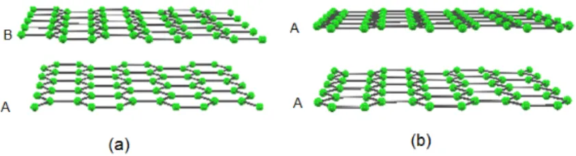
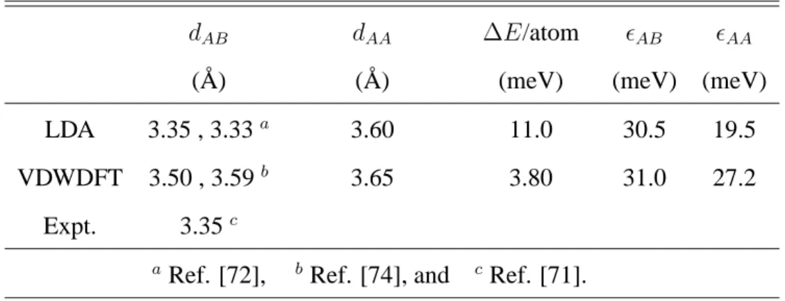
Both methods give successful results for graphite; i.e. the calculated interlayer distances are comparable with the experimental value. We find that the interlayer distance of the two-layer graphene is close to that of graphite. We also find that the AA stacking structure of the two-layer graphene has higher energy than that of the AB stacking one and the layer distance of the AA stacking is larger than that of the AB stacking. It is thus suggested that the interlayer distance becomes somewhat large when the stacking deviates from the AB stacking.
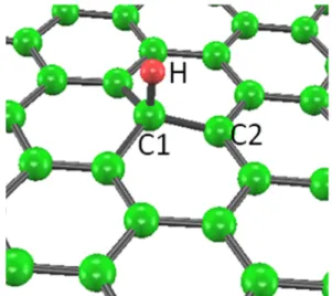
Next, we study hydrogen monomers and dimers in graphene, the armchair edge (5, 5) carbon nanotube (CNT), and the zigzag edge (10, 0) CNT because the presence of hydrogen atoms could change the electronic properties of graphenes and CNTs, where those hydrogen atoms are chemically attached. We find that the monomers in the above three carbon nanomaterials have the magnetic moment of 1µB. In the case of the CNTs, the hydrogen atoms are located on the outer side of the CNTs. In the most stable structures of the dimers in the above three carbon materials, the two hydrogen atoms are bonded to host carbon atoms, which are nearest- neighbors. In the case of graphene, the two atoms are located on opposite sides, whereas in the
i
case of the armchair edge (5, 5) CNT and zigzag edge (10, 0) CNT, both hydrogen atoms are located on the outer side. The electronic structures of the most stable geometries are found to be nonmagnetic. However, when the two hydrogen atoms are bonded to second-nearest-neighbor carbon atoms, the magnetic moment is found to be 2µB.
1. Mohammad Shafiul Alam, Jianbo Lin, and Mineo Saito: First-Principles Calculation of the Interlayer Distance of the Two-Layer Graphene: Japanese Journal of Applied Physics Vol. 50, pp 080213, August 2011.
2. Mohammad Shafiul Alam, Fahdzi Muttaquien, Agung Setiadi, and Mineo Saito: First- Principles Calculations of Hydrogen Monomers and Dimers Adsorbed in Graphene and Carbon Nanotubes: Journal of the Physical Society of Japan , vol. 82, pp: 044702, March 2013.
iii
Dedicated to my Mother
iv
Abstract i
List of Publications iii
Dedication iv
List of Figures viii
List of Tables xi
1 Introduction 1
1.1 Carbon Nano-Material . . . 1
1.2 Two-layer graphene layer distance . . . 3
1.3 Atomic hydrogen adsorption . . . 3
1.4 Purposes of this research . . . 4
1.5 Structure of the thesis . . . 6
2 Theory and Calculational details 7 2.1 Theoretical Background . . . 8
2.1.1 The variation Principle . . . 9
2.1.2 The Hartree-Fock approximation . . . 11
2.2 Density Functional Theory (DFT) . . . 14
2.2.1 Hohenberg-Kohn Theorems . . . 15
2.2.2 The Kohn-Sham equations . . . 17 v
2.3 Exchange and Correlation Functional . . . 19
2.3.1 Local Density Approximation (LDA) . . . 20
2.3.2 Generalized Gradient Approximation (GGA) . . . 22
2.4 Plane Waves Method . . . 23
2.5 Pseudopotential . . . 24
2.5.1 Norm Conserving Pseudopotential . . . 25
2.5.2 Ultrasoft Pseudopotential . . . 26
2.6 van der Waals density functional theory (VDWDFT) . . . 27
2.7 Calculation details . . . 27
3 Layer distance of the two-layer graphene 30 3.1 Results and Discussions . . . 31
3.2 Conclusion . . . 34
4 Atomic hydrogen adsorption in graphenes and CNTs 35 4.1 Graphene . . . 36
4.1.1 GGA calculations . . . 36
4.1.2 LDA calculations . . . 42
4.2 Armchair edge (5, 5) carbon nanotube . . . 46
4.3 Zigzag edge (10, 0) carbon nanotube . . . 51
4.4 Conclusions . . . 61
5 Summary 63 5.1 Conclusions . . . 63
5.2 Future Plan . . . 65
A van Der Waals Density Functional theory (VDWDFT) 66 B Hydrogen Adsorbed in Two-layer graphene 69 B.1 Results and Discussions . . . 69
B.2 Conclusions . . . 76
References 77
Acknowledgments 83
1.1 Carbon materials, (a) fullerenes, (b) nanotubes, (c) graphene and (d) graphite. . 2 1.2 Two-layer graphene having AB stacking (a) and AA stacking (b) structures. . . 3 2.1 Self-consistent scheme of Kohn-Sham equation . . . 20 4.1 Geometrical configuration of the hydrogen monomer in graphene. . . 37 4.2 Nearest-neighbor geometrical configurations of the hydrogen dimers in graphene.
A and B represent the A sublattice and B sublattice, respectively. . . 38 4.3 Charge densities of the hydrogen dimers where both of the hydrogen atoms
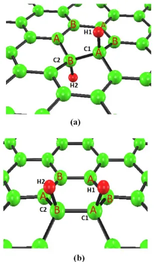
are located on opposite sides (a) and on the same side (b) of graphene. The isosurface value is 0.22(a.u)−3. . . 39 4.4 Second-nearest-neighbor geometrical configurations of the hydrogen dimers in
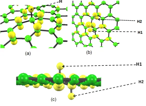
graphene. A and B represent the A sublattice and B sublattice, respectively. . . 40 4.5 Spin density distributions of the hydrogen monomer (a) and hydrogen dimer
(b, c) having second-nearest-neighbor geometry [Fig. 4.4(a)] in graphene. The isosurface value is 0.01(a.u)−3. . . 42 4.6 Geometrical configuration of the hydrogen monomer (a) and spin density dis-
tribution (b) in the graphene. The isosurface value is 0.01(a.u)−3. . . 43 4.7 Geometrical configuration of the hydrogen dimer in graphene . . . 44 4.8 Second-nearest-neighbor geometrical configuration of the hydrogen dimer in
graphene. . . 45
viii
4.9 Spin density distribution of the hydrogen dimer having second-nearest-neighbor geometry [Fig. 4.8(b)] in the mono-layer graphene. The isosurface value is 0.01 (a.u)−3. . . 46 4.10 Geometrical configurations of the hydrogen monomer in the armchair edge
(5,5) CNT [(a) and (b)], and spin density distributions of the former hydrogen monomer (c). The isosurface value is 0.01(a.u)−3. . . 48 4.11 Geometrical configurations of the pristine armchair edge (5,5) CNT (a) and the
hydrogen dimer in the armchair edge (5,5) CNT (b) and (c). . . 50 4.12 Geometrical configurations of the hydrogen dimer in the armchair edge (5,5)
CNT having the second-nearest-neighbor (a) and spin density distributions of the hydrogen dimer (b1, b2). The isosurface value is 0.01(a.u)−3. . . 51 4.13 Geometrical configurations of the hydrogen monomer in the zigzag edge (10,0)
CNT [(a) and (b)] and spin density distributions of the former hydrogen monomer (c). The isosurface value is 0.01(a.u)−3. . . 53 4.14 Density of states of the nonmagnetic electronic structure (a) and spin-polarized
electronic structure (b) of the hydrogen monomer on the zigzag edge (10,0) CNT. The energies are measured from the Fermi energy. The lower and upper lines represent the majority and minority spins, respectively. . . 55 4.15 Geometrical configurations of the pristine zigzag edge (10,0) CNT (a) and the
hydrogen dimer in the zigzag edge (10,0) CNT (b) and (c). . . 59 4.16 Second-nearest-neighbor geometrical configurations of the hydrogen dimer in
the zigzag edge (10,0) CNT (a), and spin density distributions of the hydrogen dimer (b). The isosurface value is 0.01(a.u)−3. . . 60 B.1 Geometrical configuration of the hydrogen monomer in the two-layer graphene. 70 B.2 Spin density distribution of hydrogen monomer in the two-layer graphene [Fig.
B.1(a)]. The isosurface value is 0.005(a.u)−3. . . 71 B.3 Nearest-neighbor geometrical configurations of the hydrogen dimers in two-
layer graphene . . . 72
B.4 Second-nearest-neighbor geometrical configuration of the hydrogen dimers in two-layer graphene. . . 73 B.5 Spin density distribution of hydrogen dimer having second-nearest-neighbor
configuration [Fig. B.4(b)]in the two-layer graphene. The isosurface value is -0.01(a.u)−3. . . 75
3.1 Calculated results of the graphite. dAB (dAA) represents the layer distance of the AB (AA) stacking. ∆E is the difference between the energies of the AB and AA stacking structures. ϵAB andϵAAare the interlayer binding energies of the AB stacking and AA stacking structures, respectively. . . 32 3.2 Calculated results of the two-layer graphene. dAB (dAA) represents the layer
distance of the AB (AA) stacking. ∆E is the difference between the energies of the AB and AA stacking structures. ϵAB andϵAA are the interlayer binding energies of the AB stacking and AA stacking structures, respectively. . . 33 4.1 Hydrogen monomers and dimers in graphene, armchair edge (5,5) CNT, and
zigzag edge (10,0) CNT. NN and SN denote the nearest-neighbor and second- nearest-neighbor configurations, respectively. . . 57 4.2 Hydrogen monomers and dimers in graphene. NN and SN denote the nearest-
neighbor and second-nearest-neighbor configurations, respectively. Eb is the binding energy per hydrogen atom. These results are based on the LSDA cal- culations. . . 61 B.1 Hydrogen monomers and dimers in two-layer graphene and three-layer graphene.
NN and SN denote the nearest-neighbor and second-nearest-neighbor configu- rations, respectively. Eb is the bindining energy per hydrogen atom. These results are based on the LSDA calculations. . . 74
xi
Introduction
1.1 Carbon Nano-Material
Carbon materials have various atomic structures (fullerenes, nanotubes, graphene and graphite) as shown in Fig. 1.1. Experiments and computational simulations have been carried out for revealing of their physical properties. They have been attracting much attention for the future development of nanotechnology due to the light weight, high strength, and useful properties of semiconductors [1], metals [1], half metals [2, 3, 4], superconductors [5, 6] and magnets [7, 8, 9].
We are going to focus on carbon nanotubes (CNTs) and graphene. Since CNTs were de- tected from graphite [10] in 1991, is one of the carbon allotropes with sp2 hybridization of each carbon atom. There are two kinds of CNTs, i.e; metallic CNTs and semiconducting CNTs.
CNTs have a wide range of applications. Currently, CNTs can be applied in both atomistic level and macroscopic level. In the atomistic level, CNTs have been used as atomic force microscope (AFM) tip [11]. In macroscopic level, bulk CNT can be used as a composite. CNT improved the mechanical properties of cotton fiber via the coating process [12]. Beside that, CNT also has future applications. Electronic properties of the CNT can be tuned from metallic to semi- conducting and vice versa. Therefore, CNTs can be used in semiconductor technology, for an example, CNT is used in a field-effect transistor as a substitute of silicon.
1
Figure 1.1: Carbon materials, (a) fullerenes, (b) nanotubes, (c) graphene and (d) graphite.
In 2004, long after the discovery of CNT, graphene [13] is isolated from graphite, a flat mono-layer of carbon atoms tightly packed into a two-dimensional hexagonal lattice. It is easier to obtain and cheaper in production. Graphene has been attracting a wide scientific interests because of novel electronic properties. Graphene does not have a band gap and there is so called Dirac cone at the zone bound points where the Fermi level is located. It has higher mobility than other semiconductor materials like silicon as well as high charge carrier concentrations, which makes graphene an interesting candidate for applications in electronic devices. The Nobel prize in Physics for 2010 was awarded to A. K. Geim and K. S. Novoselov ”for ground breaking experiments regarding the two-dimension material graphene”.
As mentioned above CNTs and graphenes are important materials for future electronic de- vices. In this study, we first carry out calculations of two-layer graphene to investigate layer distance. Next we focus on the calculations of atomic hydrogen adsorption in graphenes and CNTs.
1.2 Two-layer graphene layer distance
Two-layer graphene is one of the carbon materials as shown in Fig. 1.2. Nowadays, few-layer graphenes (FLG) are technologically important in semiconductor applications, due to gate con- trol of the transport properties. Recently FLG with less than ten layers each show a distinc-
Figure 1.2: Two-layer graphene having AB stacking (a) and AA stacking (b) structures.
tive band structure [14] . There is thus an increasing interest in the physics of FLGs, with or without Bernal stacking [15, 16, 17] and their application in useful devices. The electronic properties of the few-layer graphene are different from that of the single-layer graphene and this difference raises scientific problems. In the case of the two-layer graphene, for an example, electric field opening of the band gap was theoretically predicted and experimentally confirmed [18, 19, 20, 21, 22, 23]. To study the electronic properties of few-layer graphenes, it is essential to clarify the interlayer distance but the distance is still unclear.
1.3 Atomic hydrogen adsorption
As carbon nanotubes (CNTs) were detected [10] and graphene was isolated from graphite [13], comprehensive studies have been carried out with the aim of exploiting the properties of these materials. Among a variety of applications of carbon nanostructure, hydrogen storage is con- sidered strong candidate. Hydrogen is a common impurity in carbon materials. Hydrogen has a lower mass that makes more easily adsorbed and diffuses on the graphene layer which lower activation energies. Whereas the hydrogen molecules are physisorbed on carbon materials, hy- drogen atoms are chemisorbed. Chemisorption of the hydrogen atoms to the carbon atom in graphene and CNT changes the hybridization of the carbon atoms fromsp2 tosp3. Therefore,
this causes changing in atomic, electronic, and magnetic properties of the carbon material. This is very interesting because we could obtain materials with different properties, which consist of only hydrogen and carbon atoms. Thus, interactions between carbon material and hydrogen show great interest due to widely future applications.
Under atomic hydrogen atmospheres, hydrogen atoms are chemisorbed on graphene and CNTs [24, 25, 26, 27, 28, 29, 30, 31, 32, 33, 34, 35, 36, 37, 38, 39, 40]. Scanning tunneling microscopy and photoluminescence spectroscopy showed that some hydrogen atoms are chemi- cally adsorbed on carbon materials [36, 37, 38, 39, 40]. Then, first-principles calculations were performed for chemisorbed hydrogen [24, 25, 26, 27, 41, 42, 43]. Duplock et al. [28] first showed that upon adsorption of hydrogen on graphene a band gap can be opened. As a result, it became clear that hydrogen significantly affects the physical properties of carbon nanoma- terials. Hydrogen adsorption was found to affect the field emission of capped CNTs [44]. It is already well understood that atomic hydrogen adsorption may be a promising way to create magnetism [45, 46, 47]. This result indicated that the magnetism of carbon nanomaterials can be controlled by hydrogen chemisorption.
The electronic structure of hydrogen monomers in graphene has been well theoretically studied [24, 29, 48]. These theoretical studies showed that hydrogen is bonded to a host carbon atom and has a magnetic moment of 1µB [24]. For dimers in graphene, the geometry where the two hydrogen atoms are on the same side has been studied [24, 25, 33, 34]. However, as mentioned later, we find in this study that this geometry is metastable. Details of the electronic structures, including the magnetism of the monomers and dimers in the CNTs are still unclear.
1.4 Purposes of this research
As mentioned above, in section 1.2, we discuss that the layer distance of the two-layer graphene is important in the field of carbon nanomaterials and also the nearest layer interaction is van der Waals type. Therefore, in order to investigate layer distance of the two-layer graphene VDWDFT is appropriate. Moreover, in section 1.3, we also discuss that chemisorption of
hydrogen can change in atomic, electronic and magnetic properties of carbon materials. As carbon-based materials attract much attention as candidates for the future electronic devices, we study interlayer distance of the two-layer graphene and atomic hydrogen adsorption in car- bon nano-materials by simulation. Material simulation is needed to reduce of error to make a material device in the real life and also minimize enormous costs involved in any material handling project.
First we concentrate our study to find out interlayer distance of the two-layer graphene.
Recently FLGs attract wide scientific interests but little is known for the interlayer distance.
The interaction between the nearest layer is a van der Waals type. As we know conventional DFT (generalized gradient approximation (GGA)) is usually insufficient to include van der Waals interaction. GGA cannot be used for systems in which the vdW interaction makes a large contribution. We confirmed that GGA fails to reproduce interlayer distance. Therefore, van der Waals density functional theory (VDWDFT) is important to investigate interlayer distance of the two-layer graphene. Since layer distance is very fundamental physical quantity, we perform first-principles calculations. We employ VDWDFT and local density approximation (LDA).
Next we study atomic hydrogen adsorption on carbon nanomaterials. Hydrogenation is promising way to create magnetism. To understand the effect of hydrogen adsorption, the study of monomers and dimers is necessary since they are fundamental hydrogen impurities in carbon materials. There will be some difference between graphene and CNTs. To clarify the curvature effect, we study armchair (5, 5) edges CNT, zigzag edges(10, 0) CNT as well as graphene which is planar. The effects of hydrogenation in multi-layer graphenes are also considered. In this study, we report details of electronic structures, including magnetism of the monomers and dimers of graphenes and CNTs.
It is experimentally difficult to investigate the magnetic state in carbon nanomaterial by atomic hydrogen adsorption. Thus, this work is very important and significant in the field nanomaterials.
1.5 Structure of the thesis
In this thesis, the executional theories are explained in the Chapter 2. In the chapter 3, we reported our results by using a recently developed VDWDFT as well as the LDA. Both methods give successful results for graphite; i.e., the calculated interlayer distances are comparable with the experimental value. We find that the interlayer distance of the two-layer graphene is close to that of graphite. In Chapter 4, we report the study of hydrogen monomers and dimers in graphenes, the armchair edge (5, 5) carbon nanotube (CNT), and the zigzag edge (10, 0) CNT.
We find that the monomers in the above three carbon nanomaterials have a magnetic moment of 1µB. In the case of the CNTs, the hydrogen atoms are located on the outer side of the CNTs. In the most stable structures of the dimers in the above three carbon materials, the two hydrogen atoms are bonded to host carbon atoms, which are nearest-neighbors. In the case of graphene, the two atoms are located on opposite sides, whereas in the case of the armchair edge (5, 5) CNT and zigzag edge(10, 0) CNT, both hydrogen atoms are located on the outer side. However, when the two hydrogen atoms are bonded to the second nearest carbon atoms, the magnetic moment is found to be 2µB. We show spin density distributions occurred by monomers and second-nearest-neighbor dimers. Finally, I summarize this work in Chapter 5.
Theory and Calculational details
The results shown in this dissertation is based on the first-principles quantum-mechanical cal- culations. It simply says that no empirical parameters are employed in simulations to compute the electronic properties of a system, but only the atomic numbers and positions are inputs to a calculation. Due to an increase in processing power of the computer in the past few decades, it is possible to perform first-principles calculations on a larger and more realistic system. The calculations acquire a degree of accuracy, which enables direct comparison to experiments.
In this chapter, a brief overview of the theoretical methods is explained. We use the PHASE [49] calculation code. The PHASE is based on density functional theories (DFT), the pseu- dopotentials, and plane wave basis set. We explain the theoretical background in section 2.1.
In section 2.2 density functional theory is denoted. The exchange and correlation functionals, plane wave methods, and pseodopotentials are described in sections 2.3, 2.4 and 2.5, respec- tively. We explain van der Waals density functional theory (VDWDFT) and calculational details in section 2.6, and 2.7, respectively.
7
2.1 Theoretical Background
The Hamiltonian of a fully interacting system consisting of many electrons and nuclei is expressed as:
Hˆ = ˆTe+ ˆTn+ ˆVee+ ˆVnn+ ˆVext (2.1) whereTˆe, Tˆn, Vˆee, Vˆnn, and Vˆext are the many electron kinetic energy operator, many-nucleus kinetic energy operator, the electron-electron interaction energy operator, many-nucleus kinetic energy operator,and the electron-nucleus interaction energy operator, respectively.
They are expressed as following:
Tˆe =−12∑N
i ∇2i(ri) Tˆn=−12∑
j 1
Mj∇2i(Rj) Vˆee = 12∑
i̸=j
|ri−1rj|
Vˆnn = 12∑
i̸=j ZiZj
|Ri−Rj|
Vˆext=−∑
i,j Zj
|Ri−Rj|
(2.2)
where theMi,Zi, andRiare the mass, atomic number and position of the nucleusirespectively.
The Schr¨odinger eigenvalue equation of this system is given by:
HΨ =ˆ EΨ, (2.3)
where the system wavefunctionΨdepends on all configuration variable which is expresses as:
Ψ = Ψ(r1,R1,r2,R2, ...). (2.4) This equation is defined in3M+3N-parameter space, and it is too complex if not impossible to solve for all but the simplest systems.
Considering the mass of a nucleus is far from that of an electron, we can assume that the motion of the nuclei is negligible compared to that of the electrons and fix their positions. By employing this, we can neglectTˆn andVˆnn and rewrite it as a problem of many electrons in an external potentialVˆextgenerated by the stationary nuclei:
Hˆ = ˆT + ˆVee+ ˆVext, (2.5) The Schr¨odinger equation of this system is expressed as:
HΨ =ˆ [
−1 2
∑N i
∇2+1 2
∑
i̸=j
1
|ri−rj| −∑
i,j
Zj
|Ri−Rj| ]
Ψ =EΨ, (2.6)
withΨnow the many-electron wavefunction,
Ψ = Ψ(r1,r2, ...). (2.7)
This approximation method is called the Born-Oppenheimer approximation and is em- ployed in all systems that are more complex than the hydrogen atom.
We know that it is possible to find the total ground state solution if we are capable of finding the ground state solutions for fixed nuclear configurations, our problem is reduced to finding these electronic ground state solutions. For this, it is useful to introduce some additional ap- proximations, such as variation principle and Hartree-Fock approximation. Before we explain Hartree-Fock approximation, first we discuss the variation principle.
2.1.1 The variation Principle
To find any eigenfunction of the Hamiltonian operator is an impossible task, but we may con- sider all the (many-body) eigenfunctionsϕi were known. Assuming that the set of these eigen- functions is complete, we may expand any other wavefunctionsψ of the system with the same number of electrons. We, therefore, write down the following expansion.
|Ψ⟩=∑
i
ci|ϕi⟩ (2.8)
where ci are the expansion coefficients. The eigenstates |ϕi⟩are assumed to be orthonormal.
The wavefuntion is assume to be normalized, then the expectation value for the energy of the wavefunction is given by:
E =⟨Ψ|Hˆ|Ψ⟩=∑
i,j
c∗jci⟨ϕi|Hˆ|ϕj⟩=∑
i
|c2i|Ei ≥E0∑
i
|c2i|=E0 (2.9)
with E0 the lowest eigenvalue of Hˆ , i.e. the ground state energy. The expectation value of the energy of any wavefunctionψ is thus higher than or equal to the ground state energy. This result is very important as this allows us to search for the ground state wavefunction and energy by testing different ‘trial wavefunctions’. It also accepts the state corresponding to the lowest energy as the best approximation of the true ground state.
Now the problem is to find out a good trial wavefunctions. In practice, the approximate wavefunction is written in terms of one or more parameters:
Ψ = Ψ(p1, p2, ..., pN) (2.10) So, the expectation value for the energy, E, is a function of these parameters and can be minimized with respect to them by requiring that
∂E(p1, p2, ..., pN)
∂p1
= ∂E(p1, p2, ..., pN)
∂p2
=...= ∂E(p1, p2, ..., pN)
∂pn
= 0 (2.11) Let us assume that the approximate wavefunction for a given system may be expanded in terms of a particular set of plane waves. Because we cannot work with an infinitely many numbers of plane waves, we truncate the sum and just consider the first N terms:
ϕ =
∑N j
cjexp(−ik·rj) (2.12)
In order to get a good approximation ground state, we would like the above expansion to satisfy the minimum condition, i.e:
∂
∂c∗j
⟨ϕ|Hˆ|ϕ⟩
⟨ϕ|ϕ⟩ = 0 (2.13)
for eachcj. In addition, we require the approximate wavefunction to remain normalized:
⟨ϕ|ϕ⟩= 1 (2.14)
which then we can rewrite Eq.(2.13) as:
∂
∂c∗j⟨ϕ|Hˆ|ϕ⟩= 0 (2.15)
for all cj. We can satisfy Eq.(2.14) and Eq.(2.15) by introducing a new quantity which is expressed as:
K =⟨ϕ|Hˆ|ϕ⟩ −λ[⟨ϕ|ϕ⟩ −1] (2.16) and extending the minimization property to include extra parameterλ,
∂K
∂c∗j = ∂K
∂λ = 0 (2.17)
hereλ is called the Lagrange multipliers. Inserting the expansion in Eq.(2.12) into Eq.(2.17), we get
∑
j
cj
(⟨exp(−ik·ri)|Hˆ|exp(−ik·rj)⟩ −λ⟨exp(−ik·ri)|exp(−ik·rj)⟩)
= 0 (2.18) We can write in the form of a generalized eigenvalue equation,
∑
j
Hijcj =λδij (2.19)
whereHij =⟨exp(−ik·ri)|Hˆ|exp(−ik·rj)⟩andδij =⟨exp(−ik·ri)|exp(−ik·rj)⟩. We can solve these N equations (i = 1,2, ...N) by calculating the matrix elementHkj and δij. If we use N basis functions to expand the trial functionϕ, Eq.(2.12) then gives N eigenvalues. By multiplying Eq.(2.18) withc∗i and summing overiwe get the following expression;
λ=
∑
i,jc∗icj⟨exp(−ik·ri)|Hˆ|exp(−ik·rj)⟩
∑
i,jc∗icj⟨exp(−ik·ri)|exp(−ik·rj)⟩ (2.20) Eq. (2.20) implies that each of the N eigenvectors correspond to a series of expansion coeffi- cients yielding differentϕand eachλcorresponds to a different expectation value. The eigen- vector corresponds to the smallest eigenvalue then corresponds to the bestϕ and the smallest eigenvalue itself is the closest approximation to the ground state energy.
2.1.2 The Hartree-Fock approximation
A major problem with trying to solve the many-body Schr¨odinger equation is the representation of the many-body wavefunction. In 1920, Douglas Hartree [50] developed an approach named after himself called the Hartree approximation. He simplified the problem of electron-electron
interactions by expanding the many electron wavefunction into a product of single electron wavefunction which is capable of solving the multi-electron Schr¨odinger equation of the wave- function. With this hypothesis and the use of the variation principle, need to be solved N equations for an N single electrons system, with wavefunction,Ψ(ri):
ΨH(r1,r2,r3, ...rN) = 1
√Nϕ(r1), ϕ(r2), ϕ(r3), ...ϕ(rN) (2.21) whereΨ(ri)is composed of spatial wavefunctionϕ(ri).
However, the Hartree approximation does not account for exchange interaction as Eq.(2.21) does not satisfy Pauli’s exclusion principle. According to Pauli’s exclusion principle it is known that Hartree approximation fails as the Hartree product wavefunction is symmetric not antisymmetric.
We need to establish such as a reasonable approximation which has good physical meaning.
Hartree and Fock introduce an approximation method that deals with electrons as distinguish particle. In the Hartree-Fock scheme, the system with N-electron wave function is approximated by antisymmetric function.
The Hartree-Fock scheme is always described as Slater Determinant such as:
ΨHF = 1
√N!
ϕ1(r1) ϕ2(r1) · · · ϕN/2(r1) ϕ1(r2) ϕ2(r2) · · · ϕN/2(r2)
... ... · · · ... ϕ1(rN) ϕ2(rN) · · · ϕN/2(rN)
(2.22)
or in short:
ΨHF = 1
√N!det(r1)ϕ2(r2)...ϕN/2(rN) (2.23) with additional orthonormal constraint
∫
ϕ∗i(r)ϕi(r)dr=⟨ϕi|ϕj⟩=δij (2.24) With the above Slater Determinant, we can be determined the HF energy by taking the expec- tation value of the Hamitonian Eq.(2.6). It can be expressed by the given equation:
E =⟨ΨHF|Hˆ|ΨHF⟩= 2
∑N/2 i
hi+
∑N/2 i
∑N/2 j
(2Ji,j−Ki,j) (2.25)
the first term of the Eq. (2.25) indicates the kinetic energy of electrons and interaction between electrons-nuclei, then the second term represents the interaction between two electrons called Coulomb and exchange integrals, where: where
hi =
∫
ϕ∗i(r1)ˆhϕi(r1)dr1 (2.26)
Jij=
∫ ∫
ϕ∗i(r1)ϕi(r1) 1
|r1−r2|ϕ∗j(r2)ϕj(r2)dr1dr2 (2.27)
Kij=
∫ ∫
ϕ∗i(r1)ϕj(r1) 1
|r1−r2|ϕ∗j(r2)ϕi(r2)dr1dr2 (2.28) The termJijare called Coulomb integrals, which are already present in the Hartree Approx- imation. On the other hand, the exchange integralKijare represented something new. Mention that it is not necessary to exclude the term i = j from the double summation in equation Eq.
(2.25), it is becauseJij =Kij.
In order to understand in a simple way about Coulomb and exchange in Eq. 2.25, we con- siderVHF as Hartree-Fock potential. This potential describes the repulsive interaction between one electron with others N-1 electrons averagely, consists Coulomb operatorJˆand exchange operatorK.ˆ
J ϕ(r) =ˆ
∫
dr2|ϕj(r2)|2
|r1−r2|ϕi(r1) (2.29)
Kϕ(r) =ˆ
∫ dr2
ϕ∗j(r2)ϕi(r2)
|r1−r2| ϕj(r1) (2.30) In the Eq. (2.29) is called the Jˆis called the coulomb operator. In order to understand the meaning of the Coulomb operator, suppose we have two electrons in different positionsr1and r2 in such spin orbitalϕi. These electrons will repel each other, which in Hartree-Fock scheme.
The repulsive force of the first electron due to second electron is weighted by the possibility of the existence of the second electron itself at this spatial point. This Coulomb operator is called local as its expectation value only depends on the spin orbital atr1.
The termKin the Eq.(2.30) is defined exchange operator. This operator comes out to avoidˆ the self-interaction in one electron. Of course, this is an important point as it is meaningless if we had to calculate the Coulomb interaction between one electron with itself. We may call exchange operator as non local because the result of the exchange operator on an orbital, ϕi, depends on theϕi at every point in space. It is an important point that the non-local exchange operatorKˆ highlighted when we operate its with spin orbital, ie.ϕion spin: By puttingϕi(r) = ϕi(r, σ)in Eq. (2.30) we can find that the exchange interaction only affects electrons with like spins. The Hartree-Fock theory reduces the energy expectation value as electrons of like spin are kept apart. The exchange energy is the difference between the Hartree and Hartree-Fock values.
The Hartree-Fock theory does nothing to keep electrons with opposite spin away. Such electrons can interact only through the average charge density appearing in coulomb operator.
There is no pairing interaction to make it disagreeable for electrons of opposite side come together. This suggests that the ground-state energy calculated in Hartree-Fock theory is always higher than the true ground-state energyEHF > E0.
The Hartree-Fock scheme is constructed based on the effective wavefunction and potential.
We guess the first set input of Slater determinant based on Pauli’s principle for the system, so we have reasonable approximation wave function. Then we construct the potential operator with emphasizing the electron’s interaction that taken account averagely and considering the self-interaction in one electron. Next iteration is done based on the new orbitals from previous calculation until we reach the threshold point. This technique is also known as self-consistent field (SCF).
2.2 Density Functional Theory (DFT)
The Hartree-Fock equations deal with exchange exactly; however, the equations neglect more detailed correlations due to many-body interactions. The effects of electronic correlations are not negligible. The requirement for a computationally practicable scheme that successfully
incorporates the effects of both exchange and correlation leads us to consider the conceptually disarmingly simple and elegant density functional theory(DFT). Nowadays, DFT is an efficient and practical method to describe ground state properties of materials due to high computational efficiency and good accuracy. The idea of DFT is to describe interacting system via electron’s density, not wave functions. DFT is totally based on two theorems stated by Hohenberg and Kohn [51]. Here we explain the two theorems as following:
2.2.1 Hohenberg-Kohn Theorems
There are two important theorems that can be resumed from Hohenberg-Kohn work. The the- orems support us for determining the Hamiltonian operator, and the properties of the system based on electron density point of view. The electronic densityn(r)is expressed as:
n(r) =N∑
s1
...∑
sN
∫ ...
∫
|Ψ(r,s1,r2,s2, ...rN,sN)|2dr2...drN (2.31)
∫
n(r)dr =N (2.32)
Theorem I. (Hohenberg-Kohn 1, 1964) The ground state densityn(r)of a many-body quan- tum system in some external potentialVext(r)determines this potential uniquely.
Proof: Hohenberg-Kohn proved the first theorem by reducio ad absurdum. They assumed another external potential,Vext′ (r), that differed by a constant from first external potential but give rise to the same densityn(r). Now, we have two Hamiltonian operator, Hˆ and Hˆ′, that give corresponding ground wave function (Ψand Ψ′) and energies (E0 and E0′). Obviously;
these two ground state energies are different. This condition gives us a chance to use theΨ′for calculating the expectation value ofH:ˆ
E0 <⟨Ψ′|Hˆ|Ψ′⟩=⟨Ψ′|Hˆ′|Ψ′⟩+⟨Ψ′|Hˆ −Hˆ′|Ψ′⟩ (2.33) As the value of Hamiltonian are: Hˆ = ˆT + ˆVee+ ˆVextandHˆ = ˆT + ˆVee+ ˆVext′ . We can get:
E0 < E0′ +
∫
n(r)[Vext−Vext′ ]dr (2.34)
and (by changing the quantities)
E0′ < E0+
∫
n(r)[Vext−Vext′ ]dr (2.35) Then we add the Eq. (2.34) and Eq. (2.35), this summation will lead to inconsistency:
E0+E0′ < E0+E0′ (2.36) Thus the theorem proved by reductio ad absurdum
Theorem II. (Hohenberg-Kohn 2, 1964) A universal functional for the energy E[n] in terms of the density n(r) can be defined, valid for any external potential Vext(r). For any particular Vext(r), the exact ground state energy of the system is the global minimum value of this functional, and the densityn(r)that minimizes the functional is the exact ground state densityn0(r).
Proof: Since all properties such as the kinetic energy, etc., are uniquely determined ifn(r) is specified, then each such property can be viewed as a functional ofn(r), including the total energy functional:
EHK[n(r)] = T[n] +Eint[n] +
∫
vext(r)n(r)d3r+EII
= F[n(r)] +
∫
vext(r)n(r)d3r+EII (2.37) whereEII is the interaction energy of nuclei andF[n(r)]is a universal functional of the charge density n(r) because the treatment of the kinetic and internal potential energies are the same for all systems. In the ground state, the energy is defined by the unique ground state density, n(1)(r),
E0 =E[n(1)] =⟨Ψ|Hˆ|Ψ⟩ (2.38) By the variational principle, a different density,n(2)r)will necessarily give a higher energy:
E0 =E[n(1)] =⟨Ψ|Hˆ|Ψ⟩<⟨Ψ′|Hˆ|Ψ′⟩=E0′ (2.39) It follows that minimizing with respect to n(r) the total energy of the system written as a functional of n(r), one finds the total energy of the ground state. The correct density that
minimizes the energy is then the ground state density. In this way, DFT exactly reduce the N-body problem to the determination of a 3-dimensional function n(r) which minimize the functionalEHK[n(r)]. But unfortunately this is of little use asEHK[n(r)]is not known.
2.2.2 The Kohn-Sham equations
Kohn-Sham reformulated the problem in a more familiar form and opened the way to practical applications of DFT. They continued to prove the theorem which states that the total energy of the system depends only on the electron density of the system [52].
E =E[n(r)] (2.40)
An interacting electrons system is mapped in an auxiliary system of a non-interacting electrons with the same ground state charge density n(r).For a system of non-interacting electrons the ground-state charge density is represented as a sum over one-electron orbitals.
n(r) = 2
∑N i
|Ψi(r)|2, (2.41)
whereiruns from 1 toN/2if we consider double occupancy of all states.
The electron density n(r) can be varied by changing the wave functionΨ(r)of the system.
If the electron density n(r) corresponds to the said wavefunction, then its total energy is the minimized energy, and the whole system is in a ground state. The Kohn-Sham approach is to replace interacting electron, which is difficult with non-interacting electrons, which move in an effective potential [52]. The effective potential consists the external potential, and Coulomb interaction between electrons, and its effect such as exchange and correlation interactions. By solving the equations, we can get ground state density and energy. The accuracy of the solution is limited to the approximation of exchange and correlation interactions. It is convenient to write Kohn-Sham energy functional for the ground state including external potential is:
EKS = Ts[n(r)] +EH[n(r)] +EXC[n(r)] +
∫
drVext(r)n(r) (2.42) The first term is the kinetic energy of non-interacting electrons:
Ts[n(r)] = −ℏ2 2m2∑
i
∫
Ψ∗i(r)∇2Ψ∗i(r)dr (2.43)
The second term (called the Hartree energy) contains the electrostatic interaction between cloud of charge:
EH[n(r)] = e2 2
∫ n(r)n(r′)
|r−r′| drdr′ (2.44)
All effects of exchange and correlation are grouped into exchange-correlation energyEXC. If all the functional EXC[n(r)]were known, we could obtain exact ground state density and energy of the many body problem.
Kohn-Sham energy problem is a minimization problem with respect of the density n(r).
Solution of this problem can be obtained by using functional derivative as below δEKS
δΨ∗i(r) = δT[n]
δΨ∗i(r) +
[δEext[n]
δn(r) + δEH[n]
δn(r) + δEXC[n]
δn(r)
] δn(r) δΨ∗i(r)
−δ( λ(∫
n(r)dr−N)) δn(r)
[ δn(r) δΨ∗i(r)
]
= 0, (2.45)
whereλis Lagrange multiplier and The exchange-correlation potential,VXC, is given formally by the functional derivative
VXC = δEXC[n]
δn(r) (2.46)
δn(r)
δΨ∗i(r) = Ψi(r),
the last term is Lagrange multiplier for handling the constraints, so we can get non-trivial solu- tion.
The first, second, and third terms of eq. (2.45) are δT[n]
δΨ∗i(r) =−ℏ2
2m2∇2Ψi(r) (2.47)
[δEext[n]
δn(r) +δEH[n]
δn(r) +δEXC[n]
δn(r)
] δn(r)
δΨ∗i(r) = 2(Vext(r) +VH(r) +VXC(r))Ψi(r), δ(
λ(∫
n(r)dr−N)) δn(r)
[ δn(r) δΨ∗i(r)
]
= 2εiΨi(r) (2.48)
Inserting eq. (2.47), and (2.48) to eq. (2.45), we can obtain Kohn-Sham equation which satisfies many body Schr¨odinger equation.
(
−1
2∇2+VKS(r) )
Ψi(r) =εiΨi(r) (2.49) where
VKS(r) = Vext(r) +VH(r) +VXC(r) (2.50) or,
VKS(r) = Vext(r) + e2 2
∫ n(r′)
|r−r′|dr′+VXC(r) (2.51) If the virtual independent-particle system has the same ground state as the real interacting system, then the many-electron problem reduces to one electron problem. Thus we can write:
VKS(r) = Vef f(r) (2.52)
The kinetic energyTs[n(r)]is given by
Ts[n(r)] =∑
i
εi−
∫
n(r)Vef f(r)dr (2.53) By substituting this formula in equation 2.42, the total energy is given by as follows:
EKS[n(r)] = ∑
i
εi+1 2
∫ ∫ n(r)n(r′)
|r−r′| drdr′ +Exc[n]−
∫
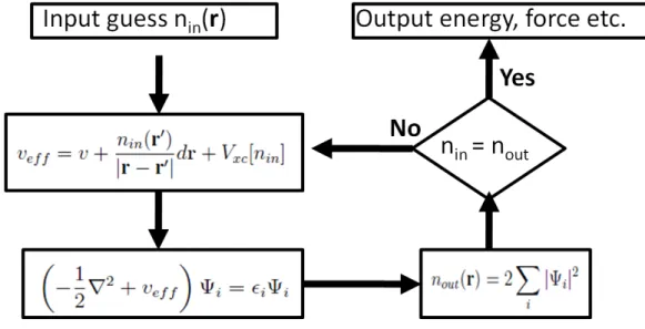
n(r)Vef f(r))dr (2.54) Since the Hartree term andVxcdepend onn(r), which depend onΨi, the problem of solving the Kohn-Sham equation has to be done in a self-consistent (iterative) way. Usually one starts with an initial guess for n(r), then calculates the correspondingVH and Vxc solves the Kohn- Sham equations for the Ψi . From this one calculates a new density and starts again. This procedure is then repeated until convergence is reached ( Fig. 2.1)
2.3 Exchange and Correlation Functional
The major problem with DFT is that the exact functionals for exchange and correlation are not known except for the free-electron gas. In previous section, the many body problems are
Figure 2.1: Self-consistent scheme of Kohn-Sham equation
rewritten to the effective one-electron problem by using the Kohn-Sham equation. But, the Kohn-Sham equation cannot be solved since the derivative EXC[n(r)] is not known. There- fore, it is very important to have an accurate XC energy functional EXC[n(r)] or potential VXC(r) in order to give a satisfactory description of a realistic condensed-matter system. For a homogeneous electron gas, this will only depend on the value of the electron density. For a non-homogeneous system, the value of the exchange correlation potential at the pointrdepend not only on the value of density atr, but also the variation close tor.
2.3.1 Local Density Approximation (LDA)
As the functionalEXC[n(r)]is unknown one has to find a good approximation for it. A simple approximation, which was already suggested by Hohenberg and Kohn, is the LDA or in the spin polarized case the local-spin-density approximation (LSDA). The exchange-correlation energy per particle by its homogeneous electron gas (HEG)eXC[n(r)]is expressed by:
ExcLDA[n(r)] =
∫
n(r)ehomoxc (n(r))dr
=
∫
n(r)[
ehomox (n(r)) +ehomoc (n(r))]
dr (2.55)
for spin polarized system
ExcLSDA[n+(r), n−(r)] =
∫
n(r)ehomoxc (n+(r),(n−(r))dr (2.56) The exchange energyex(n(r))is
eLDAx (n(r)) =− 3
4πkf (2.57)
where the Fermi wavevectorkf = (3π2n)13.
The expression of the correlation energy density of the HEG at high density limit has the form:
ec =Aln(rs) +B+rs(Cln(rs) +D) (2.58) and the density limit takes the form
ec= 1 2
(g0 rs + g1
rs3/2
+...
)
(2.59) where where the Wigner-Seitz radiusrsis related to the density as
rs= (3/(4πn))13 (2.60)
For spin polarized systems, the exchange energy functional is known exactly from the result of spin-unpolarized functional:
Ex[n+(r), n−(r)] = 1
2(Ex[2n+(r)] +Ex[2n−(r)]) (2.61) The spin-dependence of the correlation energy density is approached by the relative spin- polarization:
ξ(r) = n+(r)−n−(r)
n+(r)n−(r) (2.62)
The spin correlation energy density ec(n(r), ξ(r) is so constructed to interpolate extreme values ξ = 0,±1, corresponding to spin-unpolarized and ferromagnetic situations. The XC potentialVXC(n(r))in LDA is given by:
δEXC[n]
δn(r) =
∫ dr
[
ϵxc+n∂ϵxc
∂n ]
(2.63) VXC(r) = ϵxc+n∂ϵxc
∂n , (2.64)
EXC[n] = drn(r)ϵxc([n],r), (2.65) whereϵxc([n],r)is the energy per electron that depends only on the densityn(r).
The LDA sometimes allows useful predictions of electron densities, atomic positions, and vibration frequencies. However, The LDA also makes some errors: total energies of atoms are less realistic than those of HF approximation, and binding energies are overestimated. LDA also systematically underestimates the band gap.
2.3.2 Generalized Gradient Approximation (GGA)
The density of electron is not always homogeneous as we expected. In the case of inhomoge- neous density, naturally, we have to carry out the expansion of electronic density in the term of gradient and higher order derivatives, and they are usually termed as generalized gradient approximation (GGA). GGAs are still local but also take into account the gradient of the den- sity at the same coordinate. Three most widely used GGAs are the forms proposed by Becke [53] (B88) , Perdew et al. [54, 55], and Perdew, Burke and Enzerhof [56] (PBE). The definition of the exchange-correlation energy functional of GGA is the generalized form in Eq. (2.56)to include corrections from density gradient∇n(r)as :
ExcGGA[n+(r), n−(r)] =
∫
n(r)exc[n(r)FXC[n(r),|∇n+(r)|,|∇n−(r)|, ...]dr (2.66) Here, FXC is the escalation factor that modifies the local density approximation (LDA) expression according to the variation of density in the vicinity of the considered point, and it is dimensionless [57]. The exchange energy expansion will introduce a term that proportional to the squared gradient of the density. If we considered up to fourth order, the similar term also appears proportional to the square of the density’s Laplacian. Recently, the general derivation of the exchange gradient expansion has been up to sixth order by using second order density response theory [58]. The lowest order (fourth order) terms in the expansion ofFx have been calculated analytically [58, 59]. This term is given by the following:
FX(m, n) = 1 +10
81m+ 146
2025m2− 73
405nm+Dm2 +O(∇ρ6) (2.67)
where
m= |∇ρ|2
4(3π2)2/3ρ8/3 (2.68)
is the square of the reduced density gradient, and n= ∇2ρ
4(3π2)2/3ρ5/3 (2.69)
is the reduced Laplacian of density.
These are the comparison of GGAs with LDA (LSDA) 1. It enhances the binding energies and atomic energies, 2. It enhances the bond length and bond angles,
3. It enhances the energetics, geometries, and dynamical properties of water, ice, and water clusters,
4. Semiconductors are marginally better described within the LDA than in GGA, except for binding energies,
5. For 4d-5d transition metals, the improvement of GGA over LDA is not clear, depends on how well the LDA does in each particular case,
6. Lattice constant of noble metals (Ag, Au, and Pt) are overestimated in GGA, and
7. There is some improvement in the gap energy; however, it is not substantial as this feature related to the description of the screening of the exchange hole when one electron is removed, and this point is not taken into account by GGA.
2.4 Plane Waves Method
Plane wave methods are much more efficient than all-electron ones to calculate the atomic forces and hence to determine the equilibrium geometries. Plane waves are not centered at the nuclei but extend throughout the complete space. They implicitly involve the concept of