Viscous flow through microfabricated axisymmetric contraction/expansion geometries

Viscous flow through microfabricated

axisymmetric contraction/expansion geometries

Author Francisco Pimenta, Kazumi Toda‑Peters, Amy Q.

Shen, Manuel A. Alves, Simon J. Haward journal or

publication title

Experiments in Fluids

volume 61

number 9

page range 204

year 2020‑09‑01

Publisher Springer Nature

Rights (C) 2020 The Author(s).

Author's flag publisher

URL http://id.nii.ac.jp/1394/00001582/

doi: info:doi/10.1007/s00348-020-03036-z

https://doi.org/10.1007/s00348-020-03036-z RESEARCH ARTICLE

Viscous flow through microfabricated axisymmetric contraction/

expansion geometries

Francisco Pimenta¹ · Kazumi Toda‑Peters² · Amy Q. Shen² · Manuel A. Alves¹ · Simon J. Haward²

Received: 9 June 2020 / Revised: 5 August 2020 / Accepted: 14 August 2020

© The Author(s) 2020

Abstract

We employ a state-of-the-art microfabrication technique (selective laser-induced etching) to fabricate a set of axisymmetric microfluidic geometries featuring a 4:1 contraction followed by a 1:4 downstream expansion in the radial dimension. Three devices are fabricated: the first has a sudden contraction followed by a sudden expansion, the second features hyperbolic con- traction and expansion profiles, and the third has a numerically optimized contraction/expansion profile intended to provide a constant extensional/compressional rate along the axis. We use micro-particle image velocimetry to study the creeping flow of a Newtonian fluid through the three devices and we compare the obtained velocity profiles with finite-volume numerical predictions, with good agreement. This work demonstrates the capability of this new microfabrication technique for producing accurate non-planar microfluidic geometries with complex shapes and with sufficient clarity for optical probes. The axisym- metric microfluidic geometries examined have potential to be used for the study of the extensional properties and non-linear dynamics of viscoelastic flows, and to investigate the transport and deformation dynamics of bubbles, drops, cells, and fibers.

Graphic abstract

* Simon J. Haward [email protected] Francisco Pimenta [email protected] Kazumi Toda-Peters [email protected] Amy Q. Shen

[email protected]

Manuel A. Alves [email protected]

1 Departamento de Engenharia Química, CEFT, Faculdade de Engenharia da Universidade do Porto, 4200-465 Porto, Portugal

2 Micro/Bio/Nanofluidics Unit, Okinawa Institute of Science and Technology, Onna-son, Okinawa 904-0495, Japan

1 Introduction

Microfluidics involves fluid flows at small length scales, typically 𝓁∼100μ m (Stone and Kim 2001). Over the last two decades, the fabrication of microfluidic devices has been dominated by soft lithography techniques, which enable precise fabrication of channels with a planar rec- tangular cross-section, with complex variations of the geometry only possible in two dimensions (2D) (McDon- ald and Whitesides 2002). However, in many cases, a 2D approximation of a problem of interest is not ideal and researchers would prefer, if possible, to retain the use of the third dimension in the design of their model microflu- idic systems. A prime example is for the in vitro study of hemodynamics, which requires model blood vessels with a circular cross-section (Doutel et al. 2015; Kang et al.

2018). In addition, many processes of interest, for example spraying, inkjet printing, and fiber spinning, involve fluid flows through circular ducts and nozzles or spinnerets. In all these processes, fluid elements are subjected to exten- sional or compressional velocity gradients at locations where the cross-sectional area of a duct varies. A feature of the small length scales of microfluidics is the ability to reach high deformation rates ( ∼𝓁⁻¹ ) for relatively weak (even negligible) inertial forces (since Reynolds numbers Re∼𝓁 ) (Squires and Quake 2005). At the microscale, fluids with even weakly non-Newtonian properties such as viscoelasticity (exhibited by, e.g., blood, paints, and printing inks) can display strongly non-linear behavior due to any extensional kinematics in the flow field. This occurs due to the non-linear increase in elastic tensile stresses (or the extensional viscosity of the fluid) in regions of high strain rates and high fluid strains, resulting in feedback on the flow field. In fact, the extensional viscosity of a viscoelastic fluid often dominates the macroscopic flow response at small length scales, and is, thus, a material function of fundamental importance in a wide range of processes (Galindo-Rosales et al. 2013; Keshavarz and McKinley 2016; Haward 2016). The extensional viscos- ity of even simple Newtonian fluids is theoretically pre- dicted to depend on the mode of extensional deformation:

uniaxial, planar, or biaxial (Petrie 2006). This difference is likely to be greatly pronounced for viscoelastic fluids, so the development of axisymmetric microdevices for extensional rheometry of complex fluids is a worthwhile endeavor.

Among the various methods proposed for the meas- urement of extensional properties (or extensional rheol- ogy) of viscoelastic fluids, perhaps, the simplest is to use the extensional flow generated by a change in the cross-sectional area of the flow field. At the macroscale, there is a long history of using planar and axisymmetric

contraction/expansion geometries for examining the extensional rheology of viscous and highly non-Newto- nian fluids (e.g., Cogswell 1978; Evans and Walters 1986;

Walters and Webster 1982; James et al. 1990; McKinley et al. 1991; Rothstein and McKinley 1999; Nigen and Walters 2002). These studies show that the response of a given fluid can be significantly different in an axisym- metric compared to a planar geometry. However, to date, microscale studies (more suited to low viscosity and weakly non-Newtonian fluids) have been restricted to simple planar geometries. Initially, planar abrupt micro- fluidic contractions with a contraction ratio (the ratio of upstream to downstream channel cross-sectional area) C_r=16 were employed by Rodd et  al. (2005, 2007), while Li et al. (2011a, b) extended the study to C_r=4 and 8. The significance of C_r is that it defines the loga- rithmic (Hencky) strain on fluid elements traversing the contraction 𝜀_H=ln(C_r) . These early studies with poly- meric fluids largely focussed on the vortex growth and non-linear dynamics upstream of the contraction plane, but also demonstrated the potential of the geometry for extensional rheometry purposes. However, a major drawback of an abrupt contraction is the non-uniform velocity gradient across the contraction. This is, in prin- ciple, resolved by making a hyperbolic converging chan- nel wall profile, as described by Oliveira et al. (2007).

These authors performed Newtonian flow experiments and numerical simulations to examine the homogeneity of the extensional rate along the flow axis in converging planar microgeometries with various hyperbolic profiles.

A planar hyperbolic contraction/expansion geometry has since been commercialized as a high deformation rate extensional viscometer rheometer on-a-chip device (the e-VROC^TM , Rheosense Inc., CA, see e.g., Pipe et al.

2008; Ober et al. 2013; Keshavarz and McKinley 2016;

Garcia and Saraji 2019; Zografos et al. 2020). Similar microfluidic hyperbolic converging channels have also been employed to simulate blood flows in stenoses (Sousa et al. 2011), to measure the deformation of white blood cells (Rodrigues et al. 2015) and single DNA molecules (Larson et al. 2006), to study the deformation and breakup of droplets (Mulligan and Rothstein 2011), and to exam- ine elastic turbulence of viscoelastic fluids (Groisman and Steinberg 2000; Ekanem et al. 2020). Some of the most recent developments in this area have involved “fine-tun- ing” the hyperbolic wall profile of the planar converging/

diverging geometry by an iterative numerical optimiza- tion procedure to further improve the homogeneity of the flow field (Zografos et al. 2016). These planar optimized devices have already found applications in the study of the buckling dynamics of individual suspended actin fila- ments and for the mechanical characterization of single DNA molecules and protein aggregates (Chakrabarti et al.

2020; Liu et al. 2020). We note that it is not only the extensional viscosity of a complex fluid that is expected to depend on the applied mode of elongation. Also, since the compression/elongation in uni/biaxial extension is along two orthogonal axes (with elongation/compression along the third direction), fundamental differences can be expected in the morphologies and dynamics observed for soft objects in axisymmetric compared with planar extension (where one direction is neutral).

In this work, we aim to extend the study of microfluidic contraction/expansion flows to the axisymmetric case, which more closely represent the kinematics found in real biological systems and flow loops in general. For this, we employ a novel microfabrication technique to etch chan- nels of circular cross-section in fused-silica glass, with high precision. We begin with the relatively simple abrupt axisymmetric contraction/expansion, before examining a slowly converging/diverging hyperbolic-shaped channel.

Finally, we fabricate and test a numerically optimized geometry designed to improve the homogeneity of the extensional flow field. We examine viscous Newtonian flow in the channels using complementary experimental and numerical methods. While this is obviously a first step, nevertheless it provides a valuable characterization of the flow field for assessing the utility of such devices for purposes such as the study of the non-linear dynamics and extensional rheometry of viscoelastic fluids or the dynamics of deformable objects. Furthermore, our efforts here can lead to further advances in the fabrication of three-dimensional (3D) microfluidic devices and to more complex 3D numerical optimizations of, e.g., junctions and flow-focusing devices for applications such as droplet and fiber formation (Pimenta et al. 2018; Zografos et al.

2019). One of our ultimate goals in this line of research is the optimization of the 3D 6-arm cross-slot device, capa- ble of generating uniaxial and general biaxial extensional flows with a free stagnation point and unlimited Hencky strain (Afonso et al. 2010; Haward et al. 2012, 2019).

2 Experimental methods

2.1 Axisymmetric microfluidic devices

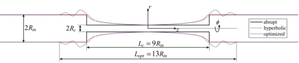
General description In this work, we employ three microfab- ricated axisymmetric geometries featuring a contraction and subsequent expansion in the cross-sectional area. The three geometries (abrupt, hyperbolic, and optimized) are shown in schematic form in Fig. 1. We define the coordinate system (r,𝜙, z) , where r is the radial position, 𝜙 is the azimuthal angle, z is the axial (streamwise) position, and the origin is located at the center of the contraction throat. For all three channels, the characteristic radius in the up/downstream in/outlets is R_in and the radius decreases to a minimum value of R_c=0.25R_in . The contraction ratio is thus C_r = (R_in∕R_c)²=16 and the Hencky strain imposed in all three channels is 𝜀_H=ln 16≈2.77.

The surface wall profile of the abrupt contraction/expansion is described by:

that is, the narrow constriction with constant radius R_c spans a length L_c=9R_in.

The hyperbolic contraction/expansion geometry converges/

diverges over the same distance of L_c=9R_in and its surface wall profile can be described as:

Since the channel cross-sectional area A(z) = 𝜋R(z)² , and for Poiseuille flow in a circular duct, the streamwise flow velocity at r=0 is v_z(z) =2Q∕A(z) (where Q= 𝜋R²_inU_in is the imposed volumetric flow rate and U_in is the average flow velocity across the inlet and outlet channels), it can be shown that the extensional rate along the flow axis of the channel

̇𝜀(z) = 𝜕v_z(z)∕𝜕z is (nominally) given by:

(1) R(z) =

{R_in : |z|>4.5R_in R_c : |z|≤4.5R_in,

(2) R(z) =

⎧⎪

⎨⎪

⎩

R_in : �z�>4.5R_in

�

R²_c

1−(0.9375�z�∕4.5Rin) : �z�≤4.5R_in .

Fig. 1 Schematic diagrams of the three axisymmetric contraction/expansion geometries, showing the coordinate system and labels for the princi- pal dimensions

Note that the nominal extension rate profile given by Eq. 3 is not expected to be entirely accurate, since it assumes that the flow fully develops instantaneously at each axial location and that there is no formation of Moffatt-like vortices (Mof- fatt 1964) in the salient corners upstream of the contraction and downstream of the expansion (Oliveira et al. 2007).

Our approach to produce a closer approximation to the nominal extension rate profile described by Eq. 3 is by the modification of the simple hyperbolic shape via numerical optimization of the channel design. The optimized channel shape is determined by the numerical procedure described in Sect. 3.1 performed over a length L_opt=13R_in (i.e., span- ning the range −6.5R_in≤z≤6.5R_in ). The resulting wall profile is complex and cannot be described by a simple piecewise function, although (as can be seen from Fig. 1) the profile collapses towards the hyperbolic shape close to z=0 . The modification of the optimized shape from the hyperbolic is mostly characterized by the bulges that appear for |z|>4.5R_in . Comparable geometric modifications were found to result from optimizations performed with planar contraction/expansion geometries (Zografos et al. 2016).

Fabrication The microfluidic devices are fabricated in fused-silica glass by the subtractive 3D-printing method of selective laser-induced etching (SLE) (Gottmann et al. 2012;

Meineke et al. 2016; Burshtein et al. 2019). SLE involves the modification of a volume of a fused-silica substrate, accord- ing to a specified 3D microchannel design, by exposure to a femtosecond-pulsed laser. Subsequently, the modified vol- ume of material is selectively removed (approximately 1000 times faster than the unmodified material) by a chemical etchant (potassium hydroxide at 80 ^◦C). The resulting micro- channels are contained within a monolithic piece of highly transparent, rigid, and chemically resistant material, capable of withstanding high pressures without deforming signifi- cantly under flow. For the channel fabrication, we employed the commercial LightFab SLE printer (LightFab GmbH, Germany), which accommodates fused-silica substrates of the size of standard laboratory glass slides ( ≈25×75 mm), and with a maximum thickness of 5 mm along the direc- tion of the light path. The instrument allows the fabrica- tion of microchannels of cross-sectional dimension down to O(10 μ m) with arbitrary 3D shapes (no limit to the angle of undercuts), and a precision and root-mean-square surface roughness of O(1 μm). We note that slight channel tapering can occur for very long channels (e.g., extending ≳10 mm from the surface inlet) due to the slow chemical etching of the un-laser-irradiated material, but this can be compensated for by introducing inverse tapering in the specified design.

(3)

̇𝜀_nom(z) =

⎧⎪

⎨⎪

⎩

0 : �z�>4.5R_in 6.67U_in∕R_in : −4.5R_in<z<0

−6.67U_in∕R_in : 0<z<4.5R_in .

Long-rectangular channels can, therefore, be fabricated fairly easily; however, due to a slightly ellipsoidal laser spot (minor axis ≈2.6μ m, major axis ≈6μ m, Meineke et al.

2016), accurate circular channels are most easily obtained in the plane normal to the laser axis. Fabricating in this direc- tion limits the maximum length of axisymmetric channel that can be etched in a single piece to around 5 mm (i.e., the substrate thickness). Accordingly, we scale our device geom- etries by setting R_in=0.36 mm, such that 13R_in<5 mm, allowing the central converging/diverging section of each geometry to be fabricated monolithically. We also fabricate 5 mm-long inlet and outlet sections of radius R=R_in , which are then bonded either side of the central piece using ultra- violet curing epoxy resin. The three pieces are carefully aligned using locating pins passing through three corners of each individual section. Photographs of each device thus fabricated are shown in Fig. 2, with the dimensions labeled.

Each photographed device is shown with the targeted wall profile superimposed in red, showing good fidelity in each case. The joins between the three individual glass pieces are visible in Fig. 2c, close to the dashed vertical lines that mark the limits of L_opt . Note that to obtain these photographs, the channels were filled with a mixture of 82 wt.% glycerol and 18 wt.% water, which has a refractive index n≈1.45 , close to that of the fused-silica substrate.

The fidelity of the fabrication to the specified design is especially critical for the optimized shape microchannel. To obtain a quantitative measure of the deviation between the fabricated channel and the specified shape, we performed an X-ray microtomography ( 𝜇-CT) scan of the channel using a Zeiss Xradia 510 Versa 3D X-ray microscope operated with the Zeiss Scout-and-Scan Control System software. For this scan, the channel was filled with a water-based contrast agent (Omnipaque 350, Daiichi Sankyo Co, Japan, at a con- centration of 350 g L⁻¹ ), which provides a strong contrast against the fused-silica microchannel substrate. The 1601 projection scan was performed with a 4× magnification objective, 100 kV voltage, 9 W power, and 4 s exposure time. The 𝜇-CT scan data were reconstructed using Amira analysis software (Thermo Fisher) and exported to Rhinoc- eros 3D modeling software (Robert McNeel and Associates) for rendering and comparison to the target profile (as pre- sented in Fig. 3). Figure 3a shows a portion of the scan data rendered by Rhinoceros. The data allow the root-mean- square surface roughness of the channel to be estimated at RMS≈0.7μ m. Line profiles along the surface of the scanned channel taken at four equally spaced azimuthal angles are plotted in Fig. 3b in comparison to the target opti- mized profile. In general, there is clearly a very good agree- ment between the channel radius measured from the 𝜇-CT scan and the specified channel design. There is an increased deviation from the design shape for |z|≳2.3 mm, which marks the location of the joins between the three assembled

glass sections. From measurements of the radius taken along the imaged channel surface at eight azimuthal angles equally spaced at 𝛥𝜙= 𝜋∕4 , we estimate the average channel radius R(z) = (1∕8)̄ ∑8

i=1R_i(z) , and, thus, the deviation from the target profile 𝛿_TAR(z) =|R(z) −̄ R_TAR(z)| . This is presented in terms of a percentage of the local target radius R_TAR(z) in Fig. 3c, (black symbols). Over the entire section of scanned channel, the deviation is ≲5% of R_TAR . The maximum per- centage deviation from the target profile occurs along the converging section of channel, close to the contraction throat ( z≈ −0.6 mm), which equates to an absolute discrepancy of

≈5μ m. The maximum absolute discrepancy from the target occurs in the outlet region z≳2.3 mm, where the 3.5% error translates to around 12μ m. We can also estimate the root- mean-square deviation of the channel from axisymmetry by comparing the measured radius at different azimuthal angles t o t h e l o c a l a v e r a g e r a d i u s 𝜎_AXI(z) =

�

(1∕8)∑8

i=1( ̄R(z) −R_i(z))² . This is also shown as a percentage of the target radius in Fig. 3c (red symbols).

Over most of the scanned length of the channel, the devia- tion from axisymmetry is <1% . There are larger deviations in the inlet ( ≈1.7% ) and the outlet channels ( ≈3.5% ), indi- cating that the three individual glass parts were not precisely aligned during assembly, resulting in a small eccentricity.

We are currently working to improve the accuracy of circular

holes fabricated in planes parallel to the light path of the LightFab laser scanner. This will enable the production of longer axisymmetric channels in a single piece of glass, and will also allow the fabrication of more elaborate geometries with interconnecting axisymmetric channels.

2.2 Flow control

To create a flow loop, tubing connectors are bonded with two-part epoxy to the inlets and outlets of the glass micro- channels and connected to 5 mL Gastight syringes (Ham- ilton, NV) via flexible silicone tubing. Flow is driven at a precisely controlled volumetric flow rate Q using two neMESYS low-pressure syringe pumps with 29:1 gear ratios (Cetoni GmbH, Germany), with one pump injecting fluid at the inlet and the second withdrawing from the outlet.

The Newtonian fluid employed in the experiments is a mix- ture of 82 wt.% glycerol and 18 wt.% water, with a density 𝜌≈1210 kg m⁻³ and a dynamic viscosity 𝜂≈56 mPa s at the temperature of the experiments ( 25±1 ^◦C). The Reyn- olds number is a function of the position in the channel:

Re=2𝜌Q∕𝜋R(z)𝜂 , which is maximal at the narrowest point, where R=R_c . For the range of flow rates applied in the experiments ( 5≤Q≤500𝜇L min⁻¹ ), the corresponding

Fig. 2 Micrographs of the three axisymmetric contraction/expansion geometries. a Abrupt, b hyperbolic, and c optimized. In each case, the specified wall profile is superimposed in red to indicate the accuracy of the fabrication

Reynolds number at the contraction throat varies in the range 0.01≲Re_max≲1 , so inertia can effectively be ignored.

2.3 Micro‑particle image velocimetry ( ‑PIV)

The flow of the Newtonian fluid through the axisymmetric microdevices is quantified experimentally using a volume

illumination 𝜇-PIV system (TSI Inc., MN). The test fluids are seeded with a low concentration ( c_p≈0.02 wt.%) of d_p =2𝜇m-diameter fluorescent tracer particles (Life Tech- nologies) with emission wavelength 𝜆=575 nm. The micro- device of interest is mounted on the stage of an inverted micro- scope (Nikon Eclipse Ti) with the z-axis parallel to the stage (i.e., horizontal), and the cross-section of the flow geometry is brought into focus with an M =4 magnification, NA=0.13 numerical aperture Nikon PlanFluor objective lens. With this setup, the depth of the measurement plane (which is normal to the direction of light propagation) over which micropar- ticles contribute to the determination of the velocity field is 𝛿m≈180μ m (Meinhart et al. 2000). Excitation with a dual- pulsed Nd:YLF laser (wavelength of 527 nm, time separation between pulses 𝛥t ) induces particle fluorescence, and a high- speed camera (Phantom MIRO, Vision Research) operating in frame-straddling mode captures pairs of particle images in synchrony with the laser pulses. At each flow rate examined, the time 𝛥t is set, so that the average displacement of particles between the two images in each pair is ≈4 pixels. All the flows in the present experiments are steady in time, so to reduce noise at each flow rate, 50 image pairs are processed using an ensemble average cross-correlation PIV algorithm (TSI Insight 4G). A recursive Nyquist criterion is employed with a final interrogation area of 16×16 pixels to enhance the spatial reso- lution and obtain 2D velocity vectors vvv= (v_r, v_z) spaced on a square grid of 16×16𝜇 m. Further image analysis, generation of contour plots, and streamline traces are performed using the software Tecplot Focus (Tecplot Inc., WA).

Since the channels are axisymmetric and have a variable radius along z, the measurement depth, 𝛿m , affects the appar- ent (measured) flow field to an extent that depends on z. For instance, at the inlet, 𝛿m≈0.5R_in but at the contraction throat ( z=0 ), 𝛿m≈2R_c . Given the Poiseuille velocity profile across the channel radius, it can be anticipated that averaging verti- cally over the measurement depth will have an increasingly significant impact on the apparent flow field as the channel radius gets smaller. The contribution of microparticles to the determination of the velocity field at the measurement plane is weighted according to the distance r from the measurement plane (only in the direction of light propagation) as defined by the following function (Olsen and Adrian 2000; Bourdon et al. 2006):

Equation 4 is an analytical expression derived by Bourdon et al. (2006), as an improvement to that derived by Olsen and Adrian (2000), for the determination of the relative weights of particles in a volume-illuminated 𝜇-PIV setup using a cross-correlation algorithm to compute velocity vectors (4) W =

[

M²d²_p+5.95(M+1)²𝜆²(n∕2NA)²+ M²r² (n∕2NA)²

]−2

.

Fig. 3 X-ray microtomography ( 𝜇-CT) of the optimized axisymmet- ric contraction/expansion geometry. a A section of the 3D-rendered 𝜇-CT scan for z>0 (diverging part). b Line profiles along the sur- face of the scan at four different azimuthal angles compared with the target (optimized) profile. Solid symbols represent z<0 (converging region) and open symbols represent z>0 (the diverging region). c Deviation of the channel profile from the target (black symbols) and from axisymmetry (red symbols), determined from measurements at eight equally spaced azimuthal angles and presented as the percent- age of the local target radius

in interrogation areas. The weighting function W (Eq. 4) is shown in normalized form in Fig. 4 alongside analyti- cal Poiseuille profiles for flow in circular channels of radius R_in and R_c (normalized by the average flow velocity in each case, U). It is clear that in the inlets and outlets of the experi- mental microfluidic devices, where R=R_in , the weighting function decays while there is only a minor variation of the expected flow profile, i.e., the measurement depth will not be expected to severely affect the determination of the flow velocity at r=0 . However, at the narrowest part of the chan- nel, where R=R_c , there is a large variation of the expected flow profile within the spread of the weighting function;

even particles located at the channel walls will contribute to the determination of the velocity field at the channel cross- section. In practice, Eq. 4 will be used in the present work to apply a depth-averaging to the numerical data that closely matches the theoretical depth-averaging of 𝜇-PIV results, thus enabling the comparison between the experimental and numerical velocity fields.

3 Numerical methods 3.1 Numerical optimization

The core of the numerical routine used to optimize the shape of the axisymmetric contraction/expansion was outlined by Pimenta et al. (2018) for planar flow-focusing devices. The routine starts with the generation of the geometry and mesh of the device, which has a deformable wall whose shape is controlled by a set of design points. After the flow has been numerically simulated, a cost function is evaluated over the axis of each trial geometry (set of design points) and fed as input to a black-box derivative-free optimizer (NOMAD, Le Digabel 2011), which generates a new trial geometry (set of design points) that attempts to reduce the cost function.

These operations are repeated in loop until the evolution of the cost function drops below a pre-defined threshold, or after exceeding a pre-defined number of iterations. In this work, the algorithm described by Pimenta et al. (2018) was adapted to the contraction/expansion geometry, which required changes in the cost function definition and in the parametrization of the deformable wall.

Geometry parametrization The parametrized axisymmet- ric contraction/expansion is depicted in Fig. 5. The geometry has radius R_in in the zone of constant cross-section, outside the optimized region. Point ‘F’ is held fixed at r=R_in and z= −6.5R_in . The 13 design points controlling the shape of the deformable portion of the bounding wall range from P₀ to P₁₂ , and form a Catmull–Rom interpolating spline. The axial coordinate of these points is fixed, whereas the radial coordinate of each point corresponds to a design variable.

The design points are uniformly distributed over the axial direction between z= −6.5R_in (point F) and z=0 (point P₁₂ ). Note that P₁₂ , the last design point at z=0 , has a modifiable radial location. Therefore, the contraction ratio is not imposed geometrically, but as will be seen next, the cost function is able to indirectly impose a pre-defined value based on mass conservation. Note also that the geometry is made symmetric in relation to plane z=0 . For creeping flow

Fig. 4 Analytical streamwise velocity profiles across circular chan- nels of radius R_in=360𝜇 m and R_c=90𝜇 m, plotted alongside the theoretical (normalized) weighting function for the contribution of particles located away from the measurement plane to the determina- tion of the velocity field

Fig. 5 Parametrized axisymmetric contraction–expansion geometry.

The radius is constant ( R_in ) outside of the optimized region. Point ‘F’

is fixed in space, whereas points P₀ to P₁₂ form a Catmull–Rom inter-

polating spline that controls the shape of the wall. The geometry is symmetric in relation to plane z=0

of a Newtonian fluid, this ensures a symmetric flow regard- ing that same plane.

Cost function The contraction/expansion geometry was optimized with the purpose of obtaining an homogeneous uniaxial extensional flow, characterized by:

in cylindrical coordinates with the z-axis aligned with the main flow direction. The extensional strain rate ̇𝜀 is posi- tive in the contraction region and negative in the expan- sion region. However, obtaining an optimized device obey- ing this condition in the entirety of its volume is a difficult task (which, for an axisymmetric device, would probably require an annular stream of lubricating fluid to avoid the no-slip condition around the channel surface, e.g., Shaw 1975; Everage and Ballman 1978; Wang and James 2011).

Rather than seeking to achieve a completely homogeneous flow field, it has been found in the case of 2D geometries more prudent to restrict the target of the optimization to the centerline of the device (Zografos et al. 2016; Pimenta et al. 2018; Haward et al. 2012; Galindo-Rosales et al.

2014), and we follow the same approach here for the 3D optimization of the contraction/expansion geometry. The flow becomes naturally extension dominated in the vicin- ity of the centerline as a consequence of the optimization procedure, but the extension is expected to be heterogene- ous (i.e., with a non-constant strain rate) approaching the wall. Nevertheless, this effect is expected to be weaker in an axisymmetric geometry than in an equivalent device with a rectangular cross-section optimized in a single direction.

This is because the Poiseuille flow profile in a circular duct is self-similar regardless of the duct radius, but the velocity profile in a rectangular channel depends upon the aspect ratio (Zografos et al. 2016). Furthermore, we reiterate that even though both the planar and the axisymmetric versions of this geometry are optimized only along the centerline, the two, nevertheless, provide fundamentally different modes of extensional deformation along that line. By limiting the tar- get of the optimization to the axis of the device (i.e., r=0 ), we, therefore, seek a device having a constant extensional rate ( 𝜕v_z∕𝜕z= ̇𝜀 =const ) in the contraction zone (defined as being over the range −z₃<z<0 ), and an equal but oppo- site extensional rate ( 𝜕v_z∕𝜕z= ̇𝜀 = −const ) in the expan- sion zone (between 0<z<z₃ ). The expected velocity and strain-rate profiles along the axis of such device are shown in Fig. 6. The velocity is symmetric and the strain rate is anti-symmetric in relation to z=0 . These are not essential conditions for our purpose, but they are desirable and they (5) vvv=

⎧⎪

⎨⎪

⎩

v_r = − ̇𝜀r∕2 v_𝜙=0 v_z= ̇𝜀z+v₀,

simply arise due to the symmetry of the geometry about the same plane and the creeping flow condition.

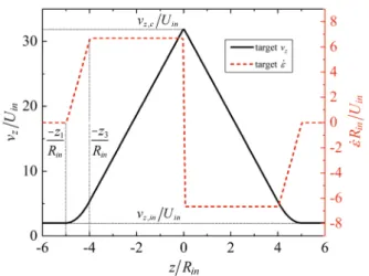
Following the approach of Zografos et al. (2016), a para- bolic velocity profile (in the region z₃ <|z|<z₁ , see Fig. 6) was introduced to connect the region of constant velocity with the extension-dominated region. This smooth transition of velocity is arguably easier to achieve numerically than an abrupt transition, leading to smaller oscillations of the velocity as a function of the streamwise position (Zografos et al. 2016). The length of the transition region 𝛥z=z₁−z₃ should be sufficient to suppress the velocity oscillations, but should also be as short as possible to maximize the region of constant velocity gradient. From a small number of pre- liminary optimizations with varying values of 𝛥z , the value of 𝛥z=R_in was selected as a reasonable compromise in this regard. The target axial velocity profile depicted in Fig. 6 is analytically described by:

where m= (v_z,c−v_z,in)∕z₂ , a=m(z₃−z₂)∕(2z₁z₃−z²

1−z²

3) , b=2az₁ , c=m(z₂−z₃) +v_z,in−az²

3+2az₁z₃ , a n d z₂= (z₁+z₃)∕2 . The average and axial velocity in the upstream and downstream non-optimized region are denoted as U_in and v_z,in (for laminar flow inside a pipe, v_z,in=2U_in ), respectively, and the axial velocity at the throat of the con- traction ( z=0 ) is v_z,c . Note that, due to axisymmetry, the radial and azimuthal velocity components vanish on the flow axis, i.e., v_r,theo(z) =v_𝜙,theo(z) =0 at r=0.

(6) v_z,theo(z) =

⎧⎪

⎨⎪

⎩

v_z,in : �z�>z₁ az²−b�z�+c : z₃≤�z�≤z₁

−m�z�+v_z,c : �z�<z₃ ,

Fig. 6 Velocity and velocity gradient profiles along the axis of the device as targeted by the numerical optimization. The velocity is constant for |z|>z₁ , follows a second-order polynomial in a transi- tion region ( z₃<|z|<z₁ ), and evolves linearly in the extension-dom- inated region ( |z|<z₃ ). The velocity profile is symmetric about z=0

The numerical optimization was carried out for z₁=5R_in , z₃ =4R_in and v_z,c∕v_z,in=16 . From mass conservation, this ratio of velocities imposes a theoretical contraction ratio of C_r=16 . This is a theoretical value, because, in practice, the radius of point P₁₂ , at the throat of the contraction, is a design variable, which, however, tends to R_in∕4 as the cost function is minimized.

The cost function is defined as:

for each trial geometry, i.e., for each vector {r_i}_i=0...12 , where v_z,num is the velocity profile sampled over the axis of the trial geometry and N is the number of sampling points (typically, N=100 ), which are kept fixed in space independently of the geometry.

Flow solver The velocity field was obtained from the solution of the steady-state Navier–Stokes equations for a Newtonian fluid in the Stokesian limit ( Re→0 ). The equa- tions were solved with a second-order finite-volume method, using rheoTool (Pimenta and Alves 2016, 2017). A mesh dependence study was carried out to ensure the space con- vergence of the results presented in this work.

4 Results

In this section, we present the results of experimental flow velocimetry and finite-volume numerical simulations for vis- cous Newtonian fluid flow through the three axisymmetric contraction/expansion geometries. The experiments are car- ried out at low Reynolds numbers ( Re_max≲1 ) and the simu- lations are performed in the Stokesian creeping flow limit ( Re→0 ). In all the results presented subsequently, lengths are normalized by R_in and velocities are normalized by U_in . Normalized quantities are specified by a superscript ‘*’.

4.1 Abrupt contraction/expansion

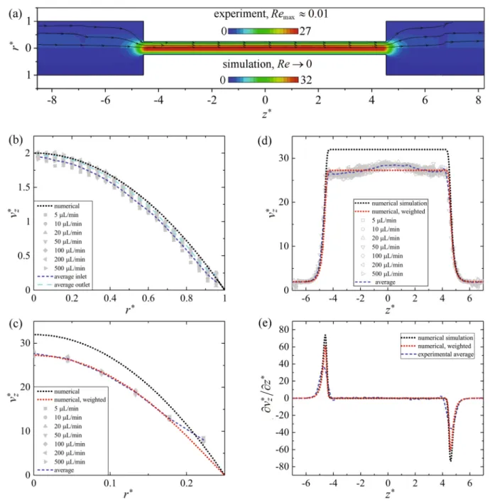
Results obtained from the abrupt contraction/expansion geometry are presented in Fig. 7. In Fig. 7a, we show a side-to-side comparison between the experimental (top) and numerical (bottom) velocity fields for creeping Newto- nian flow over the whole contraction/expansion region. Note that in the experiment (here shown for Q=5𝜇 L min⁻¹ , Re_max≈0.01 ), due to the available field of view at 4× magni- fication, three separate measurements are required to capture the displayed range of z^∗ . The three obtained fields are subse- quently assembled manually to obtain the top half of Fig. 7a.

Note also the different range of the color scales (representing the normalized velocity magnitude |vvv^∗| ) between the experi- ment and the simulation. This is due to the apparently lower

(7) C{r_i}_i=0…12=

∑N j=0

||||v_z,num(z_j) −v_z,theo(z_j) v_z,theo(z_j) ||

||

experimental velocity in the narrow constriction, which is a result of the increased importance of the measurement depth in the lower radius section of channel (as explained in Sect. 2.3). In Fig. 7b, we show the profiles of the streamwise flow velocity v^∗_z as a function of the radial position across the channel upstream of the contraction ( z^∗≈ −8 ) and down- stream of the subsequent expansion ( z^∗≈8 ). The experi- mental data from different imposed flow rates (all Re_max≲1 ) collapse well, as expected, and the profiles compare well with numerical profiles for fully developed Poiseuille flow in a circular pipe. Figure 7c shows the profiles of v^∗_z as a function of r^∗ across the narrow section of channel close to z=0 . Since the narrow section of channel has a con- stant radius R_c , for smoothing purposes the profiles shown in Fig. 7c are, in fact, obtained by averaging the velocity over a section of the channel between −2.5≲z^∗≲2.5 . Here, the experimental profiles for different imposed flow rates also collapse well, but they are significantly lower than the numerical prediction. However, we find that by applying the weighting function (Eq. 4, Fig. 4) to the numerical data, we obtain a weighted numerical profile (shown by the dotted red line) that closely matches the experimental measurement.

This shows that the true flow velocity in the narrow section of the axisymmetric microchannel is, in fact, in good agree- ment with expectations.

In Fig. 7d, we examine the streamwise fluid velocity along the length of the flow axis (along r=0 ). The experi- mental data at different flow rates collapse as expected and, upstream of the contraction plane, the flow velocity has a constant value v^∗

z,in≈2 . Approaching the contraction plane, the flow accelerates sharply to reach a constant value inside the constriction. This is predicted to be v^∗_z,c=16v^∗_z,in=32 , due to the contraction ratio C_r=16 . In the experimental measurement, v^∗_z,c appears to be rather lower than expected, but this is accounted for by the measurement depth of the 𝜇-PIV setup, as shown by the weighted numerical predic- tion (dotted red line). On passing the expansion plane, the flow decelerates into the outlet channel back to a velocity v^∗_z,in≈2 , forming a curve that is rather symmetric about z=0.

The streamwise velocity gradient (or extensional strain rate 𝜕v^∗_z∕𝜕z^∗= ̇𝜀^∗ ) along the centerline axis is shown in Fig. 7e. Here, to reduce scatter resulting from taking pointwise spatial derivatives of noisy data, the experi- mental curve (blue dashed line) is computed from the average of all the experimental data shown in Figure 7d.

The extension rate profile in the abrupt axisymmetric con- traction/expansion geometry is characterized by a positive spike of width 𝛥z^∗∼1 , reaching a peak of ̇𝜀^∗ ≈80 at the contraction plane, followed by an anti-symmetric spike at the downstream expansion plane. Clearly, there is no lengthscale over which the extensional rate can be mean- ingfully described as uniform or homogeneous, which

is a necessary requirement of an extensional rheometer.

However, abrupt changes in the cross-sectional area of axisymmetric ducts are commonplace in real flow loops used in, e.g., biomedical and industrial systems involving viscoelastic fluids. It will be interesting and instructive

to study the non-linear dynamics of such flows (e.g., McKinley et al. 1991; Rothstein and McKinley 1999) in an axisymmetric microfluidic system using modern visu- alization and measurement techniques.

Fig. 7 Experimental and numerical results for viscous fluid flow in the axisymmetric abrupt contraction/expansion geometry. a Experi- mental flow field with superimposed streamlines measured at a low Reynolds number by 𝜇-PIV (top half), and the numerically simulated flow field for creeping flow (bottom half). Color scale bars indicate

|vvv^∗| ; b normalized experimental velocity profiles across the radius of the channel inlet ( z^∗≈ −8 ) and outlet ( z^∗≈8 ), compared with the numerical prediction for fully developed flow; c normalized flow pro-

files across the radius of the narrow section of channel ( z=0 ) com- pared with the result of the numerical simulation and also weighted average of the numerical result accounting for the measurement depth of the experiment (see Eq. 4); d normalized flow profiles along the channel axis (i.e., r=0 ) compared with the numerical simulation and the weighted numerical result; e normalized extensional strain rate along the channel axis, computed by taking derivatives of the data shown in part (d)

4.2 Hyperbolic contraction/expansion

The results of the experiments and numerical simulations in the axisymmetric hyperbolic contraction/expansion geom- etry are summarized in Fig. 8. A side-to-side comparison between the experimental (top) and numerical (bottom) creeping Newtonian flow fields is provided in Fig. 8a. As

for the abrupt geometry described previously, due to the limited field of view in the 𝜇-PIV setup, the experimental field presented in Fig. 8a is an assembly of three separate measurements made at different z regions. Also note the reduced range of the velocity magnitude color scale for the experiment, which is due to the effect of the 𝜇-PIV measure- ment depth. Nevertheless, there is obviously a rather good

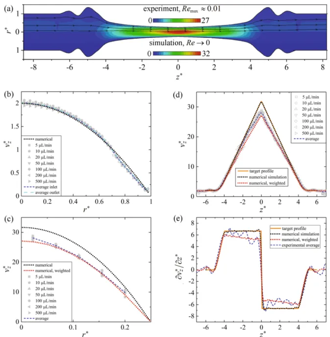
Fig. 8 Experimental and numerical results for viscous fluid flow in the axisymmetric hyperbolic contraction/expansion geometry. a Experimental flow field with superimposed streamlines measured at a low Reynolds number by 𝜇-PIV (top half), and the numerically simulated flow field for creeping flow (bottom half). Color scale bars indicate |vvv^∗| ; b normalized experimental velocity profiles across the radius of the channel inlet ( z^∗≈ −8 ) and outlet ( z^∗≈8 ), compared with the numerical prediction for fully developed flow; c normal-

ized flow profiles across the radius of the narrow section of channel ( z=0 ) compared with the result of the numerical simulation and a weighted average of the numerical result (see Equation 4); d normal- ized flow profiles along the channel axis (i.e., r=0 ) compared with the numerical simulation and the weighted numerical result; e nor- malized extensional strain rate along the channel axis, computed by taking derivatives of the data shown in part (d), and compared with the nominal strain rate given by Eq. 3

agreement between the experiment and the simulation. The apparent good agreement is confirmed by taking profiles of the streamwise flow velocity ( v_z(r) ) at locations across the channel inlet and outlet (at z^∗ ≈ −8 and z^∗≈8 , Fig. 8b) and across the contraction throat ( z=0 , Fig. 8c). The experi- mental data at different flow rates collapse well at the low imposed Reynolds numbers ( Re_max≲1 ). Across the inlet and outlet, the 𝜇-PIV measurement depth has an almost neg- ligible effect on the velocity measurement. The experimen- tal profiles agree very well with the numerical prediction (Fig. 8b), indicating that the flow is fully developed before the start of the converging region and redevelops fully in the outlet channel. Across the contraction throat (Fig. 8c), the increased significance of the measurement depth causes a reduction in the measured flow velocity below the numerical prediction. However, as was the case in the narrow section of the abrupt contraction/expansion geometry, weighting the numerical prediction using Eq. 4 results in a better agree- ment with the experiment.

In Fig. 8d, we present the streamwise fluid velocity v_z(z) along the centerline axis. The experimental data at different flow rates collapse as expected and are mostly well described by the weighted numerical prediction. The flow veloc- ity at the contraction throat ( z=0 ) is a little higher than given by the weighted numerical prediction (also evident at r=0 in Fig. 8c), which probably indicates a small error in the channel dimension at that point. It can be estimated that the higher experimental flow velocity at z=0 would be accounted for if the fabricated geometry had a radius R_c≈87.5𝜇 m at the contraction throat, i.e., just ≈2.5𝜇 m smaller than intended. We observe good symmetry of v_z(z) about the plane z=0.

Figure 8e shows the streamwise velocity gradient ( 𝜕v^∗_z∕𝜕z^∗ = ̇𝜀^∗ ) along the axis of the hyperbolic channel. The derivative computed from the average of all the experimen- tal data (dashed blue line) is shown in comparison with the numerical prediction (black dots), the weighted numerical prediction (red dots), and the nominal value of ̇𝜀 expected in this geometry, given by Eq. 3 (gray solid line). Considering the inevitable noise in the experimental profile, it is obvious that the fabricated geometry performs well in comparison with the numerical predictions. Approaching the hyperbolic region from upstream, the data show that the velocity gradi- ent begins to increase ≈1R_in before the start of the converg- ing section and that the nominal value of ̇𝜀^∗_nom=6.67 is only reached after a distance of about 1R_in within the converging part of the channel. In the downstream expansion region, an anti-symmetric behavior is observed. Despite the clear discrepancy from the ideal behavior near the start/end of the hyperbolic-shaped converging/diverging regions, an approximately uniform extensional rate is achieved by the geometry over a substantial length either side of the contrac- tion throat. The numerical simulation indicates that, within

the hyperbolic part of the microchannel, ̇𝜀 remains within 1%

of the nominal value between 0.29≤|z^∗|≤3.01 and within 5% of the nominal value between 0.22≤|z^∗|≤3.75.

4.3 Optimized contraction/expansion

In this subsection, we discuss the results of experiments and numerical simulations performed in the optimized shape contraction/expansion geometry, which was numerically designed with the intention to improve the homogeneity of the extensional flow field generated along the axis of the hyperbolic converging/diverging channel. A comparison between the creeping Newtonian flow field obtained experi- mentally (top half) and numerically (bottom half) is shown in Fig. 9a. A very good qualitative agreement is observed, subject to the same caveats given previously for the abrupt and hyperbolic contraction/expansion geometries.

As before, we extract experimental velocity profiles of v_z(r) across the inlet ( z^∗≈ −8 ) and outlet ( z^∗≈8 ) channels (Fig. 9b), which, by comparison with the numerical predic- tion, indicate that the flow is fully developed both upstream and downstream of the optimized section of channel. Across the contraction throat ( z=0 ), the experimental v_z(r) pro- file is in reasonable agreement with the weighted numerical prediction (Fig. 9c), as was also the case for the abrupt and hyperbolic channels discussed above.

The streamwise velocity profile ( v_z(z) along the cen- terline) in the optimized geometry is shown in Fig. 9d. In general, the experimental data are well described by the weighted numerical prediction. The measured flow veloc- ity is slightly higher than expected at z=0 , but the differ- ence is accounted for by the small ( ≈1% ) discrepancy from the target shape at this location (see Fig. 3c). We also note some skewness of the experimental data about z=0 , with slightly higher velocities at z<0 than at z>0 . This can also be accounted for by the deviation of the actual channel shape from the design, which, as can be seen in Fig. 3b,c, is slightly narrower than the target at z<0 , but is closer to the target at z>0.

Figure 9e shows the streamwise velocity gradient ( 𝜕v^∗_z∕𝜕z^∗= ̇𝜀^∗ ) along the axis of the optimized channel.

It is once again clear that, notwithstanding noise in the experimental data, the fabricated device performs well in comparison to the numerical simulation. Furthermore, the numerical simulation follows the target profile of the optimi- zation very well. In this case, we find that the velocity gradi- ent remains within 1% of the nominal value ( ̇𝜀^∗_nom=6.67 ) between 0.57≤|z^∗|≤3.48 and within 5% of the nominal value between 0.17≤|z^∗|≤4.05 . These approximately homogeneous regions of extensional flow are 7.0% and 9.9%

(respectively) larger than those found in the simpler hyper- bolically profiled channel.

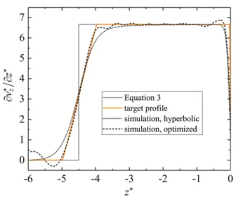
The effect of the optimization on the resulting streamwise velocity and velocity gradient profiles compared with the hyperbolic case is subtle and is not very clear by comparing Figs. 8 and 9. Accordingly, we present a direct comparison between the velocity gradient profiles obtained from the hyperbolic and the optimized geometries in Fig. 10. Here, for clarity, we only show profiles resulting from the numerical

simulations compared against the nominal profile described by Eq. 3 and the target profile of the numerical optimiza- tion. Also, since all the profiles are anti-symmetric about z=0 , we only show the converging region of the geometry to obtain a more enlarged and detailed view of the salient features. It is evident that the optimization introduces some oscillations into the velocity gradient profile, particularly

Fig. 9 Experimental and numerical results for viscous fluid flow in the axisymmetric optimized contraction/expansion geometry. a Experimental flow field with superimposed streamlines measured at a low Reynolds number by 𝜇-PIV (top half), and the numerically simulated flow field for creeping flow (bottom half). Color scale bars indicate |vvv^∗| ; b normalized experimental velocity profiles across the radius of the channel inlet ( z^∗≈ −8 ) and outlet ( z^∗≈8 ), compared with the numerical prediction for fully developed flow; c normal-

ized flow profiles across the radius of the narrow section of channel ( z=0 ) compared with the result of the numerical simulation and a weighted average of the numerical result accounting for the measure- ment depth of the experiment (see Eq. 4); d normalized flow profiles along the channel axis (i.e., r=0 ) compared with the target profile of the optimization (Eq. 6), the numerical simulation and the weighted numerical result; e normalized extensional strain rate along the chan- nel axis, computed from the data shown in part (d)

upstream of the converging region where the large bulges appear in the wall profile of the optimized geometry. The main effect of the bulges in the optimized geometry is to delay the increase in the velocity gradient of the flow until further downstream compared with the hyperbolic case.

The increase in the velocity gradient then occurs over a shorter length in the optimized geometry, more efficiently approaching the nominal value inside the converging region

̇𝜀^∗_nom=6.67 . Similar observations were made by Zografos et al. (2016) for flows in optimized planar contraction and expansion geometries.

5 Discussion

In this work, we have examined viscous fluid flows through several axisymmetric microfluidic geometries featuring contractions and expansions, which can be useful for gen- erating extensional flows and for modeling aspects of vari- ous biological and industrial fluid processing applications.

Selective laser-induced etching (SLE) was used to fabri- cate the geometries in fused-silica glass and micro-particle image velocimetry ( 𝜇-PIV) was used to experimentally measure the velocity fields inside the channels under con- ditions of laminar flow (Reynolds number, Re≲1 ). We began by fabricating and testing a canonical microfluidic abrupt axisymmetric contraction/expansion, which per- formed in accordance with the predictions of finite-vol- ume numerical simulations. Such devices are important due to their ubiquity in real-life flow loops, but do not generate a homogeneous extensional flow field (which

is a key requirement for applications such as extensional rheometry). Next, we examined a contraction/expansion geometry with hyperbolic converging/diverging regions, which can be expected to provide a nominally uniform extensional rate anticipated to be useful for extensional rheometry. The fabricated device was again shown to perform as expected on the basis of numerical simulation and did, indeed, produce a uniform elongation rate over a significant proportion of the hyperbolic profile. Finally, we attempted to improve the hyperbolic shape by carry- ing out a numerical optimization of the geometry. The resulting complex axisymmetric geometry was fabricated by SLE and tested experimentally, again with good perfor- mance. The numerically optimized shape provided some improvement on the homogeneity of the extensional flow field compared to the hyperbolic geometry. However, the O(10%) increase in length over which the extension rate remained approximately uniform perhaps does not repre- sent a substantial improvement in performance. In planar microfluidic devices, the advantage of numerical optimi- zation techniques seems to be more evident in multiple- stream devices such as T-junctions and X-junctions (e.g., Pimenta et al. 2018; Zografos et al. 2019; Haward et al.

2012; Galindo-Rosales et al. 2014), for which it is inac- curate to compute an analytical shape based on simple methods. The same is likely to also be the case in axisym- metric devices.

In many cases, axisymmetric microfluidic geometries can provide a closer representation of a process than the 2D planar (rectangular) microchannels often used, but they are challenging to fabricate and to make measurements inside of. We have shown that SLE is a viable method for the accu- rate production of axisymmetric microdevices with com- plex shape profiles and we have demonstrated that optical probes (here 𝜇-PIV) can be used to precisely measure the flow inside such devices. In this work, we have focused on developing axisymmetric microdevices designed to impose uniaxial and biaxial extensional kinematics to fluid elements.

The radial compression and stretching of fluid elements dif- fers fundamentally from the planar extensional kinematics generated in a rectangular channel. Our new devices may find uses in studying the deformation of fibers, drops, bub- ble, or cells in uniaxial extensional and compressional veloc- ity gradients, where morphological dynamics will certainly differ from those observed in planar flows. The hyperbolic and optimized shaped axisymmetric geometries may also find applications in the non-linear dynamics and extensional rheometry of complex fluids, which are also expected to vary depending on the mode of extensional deformation.

In future, we plan to study complex fluid flows (polymer solutions or suspensions) in these devices. We also intend to try optimizing other 3D geometries such as flow-focusing microdevices based on coannular channels, and ultimately

Fig. 10 Numerical extensional rate profiles along r=0 for the hyper- bolic and optimized contraction/expansion geometries. The simula- tion results are compared against the nominal extension rate profile given by Eq. 3 and the target profile of the optimization procedure given by Eq. 6