Multidimensional Scaling of Preference Data by a Unfolding Model with Multiple Ideal Points

Many model have been proposed to analyze preferenee data in several fields of research. Green and Rao discussed on how to analyze this type of data. Coombs proposed the unfolding model with ideal point and Carroll proposed the preference mapping models in frame of individual differences. The degree of the preference is assumed to be represented by a single-peaked preference function in the individual differences models in the preference. This assumption for the preference function is not appropriate to analyzing some data, for example, the preference of tea on the dimension of temperature. And we propose the unfolding model with multiple ideal points in this paper. In this model, we assume that there are two or more ideal points for each individuals when he / she evaluates the preference to the objects. First, a model is proposed. Second, an non-metric procedure is introduced. An estimation procedure using gradient method is also presented. An application to the real data set is shown. Some extension of the proposed model is discussed.

 選好度データを分析するためのモデルの一つとして理想点モデルがある。このモデルでは、個人と ものからなる２相２元選好行列について、観測された選好度と、理想点とものを表す点との点間距離 が対応づけられるように、 これらの個人と対象を点として埋め込むモデルである。従来のモデルでは、

選好度関数として単峰性関数を想定している。しかし、例えば、紅茶の温度についての好みについて 選好度データでは、理想的な温度が２個あると想定したモデルがより適切であると考えられる。本論 文では、そのような場合へも適用できるように、従来の理想点モデルの拡張を提案する。また、実際 のデータへの適用についても述べる。

Unfolding model, Preference data, Multiple ideal points.

展開法、選好データ、多重理想点

Multidimensional Scaling of Preference Data by a Unfolding Model with Multiple Ideal Points

Tadashi Imaizumi

１ Introduction

Preference data are often collected in several fields of behavioral sciences. Preference data shows the degree of preference to each of n objects, such as foods items, of each individual of N individuals. Hence, this is two-mode two-way N × n matrix. When we collect data as paired comparison data, this data matrices is two-mode three-way N × n × n matrices. We can find the hidden structure of data by fitting some models to the given preference data. Green and Rao[1] showed several examples of these data and discussed on how to analyze.

Thustone[2] proposed the law of comparative judgment for the paired comparison data. Luce[3] proposed the deterministic probablity model so called Bradley-Terry- Luce(BTL) model. These models aims to scale n objects on unidimensional space.

Coombs[4] introduced the nonmetric unfolding model, the I scale and J scale.

Bennett and Hays[5] generalized Coomb’s unidimensional unfolding model to multidimensional cases. In those models, individuals and objects are represented as points in p-dimensional Eulidean space such ans the observed rank of preference values are connected to the distance between point of individual and point of lbjects, respectively. Schönemann[6] derived an algebraic solution for the metric unfolding model. Carroll[7] contributed by the models for individual differences in the preference data. These models and procedures are to represent individuals and objects as points in multimensional space. There are other approach to analyze the preference data as realization of random variables on the degree of preference.

Schönemann and Wang[8] proposed the individual differences model of preference data. Zinnes and Griggs[9] proposed a probabilistic model and method based on the assumption of normality of points. De Sarbo and Rao[10] proposed the general unfolding models.

hese models are basically introduced by unfolding model with ideal point. In the simple unfolding model, each object of n objects is represented as a point in p- dimensional Euclidean space. And each individual is represented as a point, which is called as ideal point, in that space. Preference of individual i to a object j, pr f ij , is linke with the distance d ij

d ² ij ＝ || y i - x j || (1) where y i is the dieal point of individual i, x j is the point of object j in p-dimensional Euclidean space respectively. This model assumes that the degree of the preference is decreased as the distance from the ideal point to object increases. Carroll[7]

discussed on the individual differences in the preference data, the internal analysis and the external analysis of this type of data. He also discussed on the different case, in which the degree of the preference is increased as the distance from the ideal point to object increas3es, and proposed an unfolding model with negative weights. Carroll characterized the different property of the preference data, the single-dipped preference function in his proposal. Srinivasan and Shocker[11]

suggested this type of preference function to be needed and commented on other

models will not be appropriate model to some data. When we ask the preference of tea on the dimension of temperature for each of N individuals, some individuals will have two peaked preference function. One peak is on cool temperature and the other is on hot temperature. Such preference data will be expressed by introducing that the preference function is multiple peaked preference function.

This means(1) that there are many ideal points for each individual, and (2) that a or some ideal points determines the preference. In this paper, we suppose that each individual has one or more ideal points, and that the degree of preference to one of n objects is connected with distances from these ideal points to one of n points of objects. By introducing this multiple ideal points for each individual, this data will be explained.

２ Model

Let there be N individuals and n objects, and pr f ij denote the degree of preference of individual i(i＝1, 2, …, N), to object j (j＝1, 2, …, n). We assume that (1) each object of n objects is represented as point in p-dimensional Euclidean space, (2) and each individual of N individuals has m ideal points in that space.

(3) And we also assume that pr f ij is monotonically decreasing with the distance d ~ ij ,

pr f ij ＝M i (d ~ ij ), (2)

where

d ~ ij ＝min ( 1 d ij , 2 d ij ,…, m d ij ), (3)

k d ij ＝  Σ( k y it - x jt ) ² ,  k＝1,…,  m, (3)  

k y it is the coordinate of the k -th ideal point k y it for individual i on the dimension t and x jt is the coordinate for object j on the dimension t. The preference value of individual i to object j is monotonically decreasing function of minima of m distances from each ideal point.

By the number of ideal points, there are mainly two sub models of the model proposed.

2.1 Number of ideal points is one for all individuals

This model will be specified as m ＝1 and is corresponding to the original unfolding model. In this model, the preference function is the single peaked one which peaked at d ij ＝0. Figure 1 shows an example of preference function. The vertical axis represents the preference value, which is defined by 7 - d ij , from ideal point with coordinate (x, y) ＝  (4.5, 3) on the 2-dimensional Euclidean space.

p

t =1

Fig.1 An example of simple Unfolding Model

2.2 Multiple ideal points for all ideal points

We assume that the preference function is multiple peaked preference function.

Each individ ual has same isopreference contours from his/her ideal points. Figure 2 shows an example of preference function from two ideal points with coordinates (4.5, 3) and (-4.5, 0) of 2-dimensional Eulidean space, respectively. And the preference values are defined by 7-min ( 1 d ij , 2 d ij ).

Fig.2 An example of the Preference function when the Number of Ideal Points is two

2.3 Nonmetric scaling of preference values

We assume the preference data are collected on the ordinal scale value at least for each individual. This means that data are row conditional data.

pr f ij ＝M i (d ~ ij ) (5)

The other potion on data comparion will be matrix conditional, which means,

pr f ij ＝M (d ~ ij ) (6)

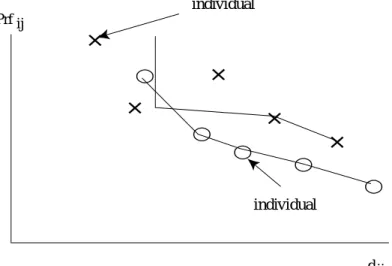
Figure 3 and 4 show the functional relationship between pr f ij and d ij when data is row conditional or matrix conditional, respectively. Segmented lines in these Figures show the monotonously transformed value of d ij by Kruskal’s principle[13]

Fig.4 An example when Preferece Data is Matrix Conditional.

Fig.3 An example when Preferece Data is Row Conditional.

×

×

×

×

×

◯

◯

◯ ◯

◯ individual

individual Prf ij

d ij

×

×

×

×

×

◯

◯

◯ ◯

◯ individual

individual Prf ij

d ij

３ The  Algorithm

We assume the degree of the preference being at least the ordinal number. A nonmetric algorithm to derive the configuration (x jt ; j ＝1,…, n, t ＝1,…, p), ( k y ik ; i ＝1,…, N, t ＝1,…, p, k, k ＝1, …, m) by analyzing two-mode two-way preferences pr f ij (i ＝1,…, N, j ＝1,…, n) among n objects from N individuals will be presented.

The measure of badness-of-fit between d

ij and the monotone transformed pr f ij , called stress S, is based on the Stress Formula 2 (Kruskal and Carroll [14] and defined as

S ＝  ΣS ² i /N, (7)

where S i is the measure of badness-of-fit for individual i,

＾

~ ~

S ² i ＝   Σ ⁿ j=1  (d ij - d ij ) ²

, (8)

                  _~

_~

      Σ ⁿ _j=1  (d ij - d i ) ²

＾

~ ~

where d ij is the transformed value of d ij defined by Kruskals monotone algorithm[13]

and

＾

  ~ ~

d ij ＝Σd ij /n (9)

which represents the mean of d ~ ij for individual i. The stress S is a function of x jt and k y it . The problem here is to find x jt , and k y it which minimize S in a Euclidean space of a given dimensionality. The iterative algorithm to minimize S is based on the steepest descent method.

3.1 Summary of the algorithm

As illustrated in Figure 5, the algorithm has three segments. The first segment is reading preference data and constructing initial configurations. The second is the iterative process which minimizes S in a Euclidean space of a given dimensionality p; and the third is obtaining the principal axes solution of the resultant configurations.

The iterative process consists of (a) updating X＝ [x it ], and (b) updating Y＝ [ k y it ].

At each iteration, S is calculated to check for convergence. If not, a new iteration begins. If no further iterations and needed, the iteration is terminated. When S becomes small enough to be neglected or the difference between S of the present iteration and that of the previous iteration becomes negligible, it is judged that S converged.

N

t =1

n

t =1

Start

Read Preferenoe Matrix

Convert this preference to a scalar product matrix by double centering it

Is the higher dimensional results available ?

Begin the iterative process

Normalize X and Y

Calculate S

Update X

Normalize X and Y

Update Y

End of the iterative process

Rotate (X,Y) into the principle axes solution

The dimensionality is minima

End Is further iteration process

needed ?

Use the first p dimensions of X and Y as the initial configurations of X

Decompose the scalar product matrix by SVD. Use these two matrix as the rational initial configrations X and 1

Set the second 2

=0

Generate K Y radomly for K=3,4, ...m 1

2

2 1

No

No Yes

Yes

No

No Yes

Yes m>2

Fig.5 Flow chart of the algorithm

3.2 Initial configurations

Constructing initial configurations for given X and Y depends on whether a higher dimensional result of the analysis of the same data is available. When the higher dimensional result is available, initial configurations can be derived from it. When the higher dimensional result is not available, the initial configuration X and Y is derived from the observed preference data. The preference matrix is then converted to a scalar product matrix by double centering the matrix. A p-dimensional configuration of objects and individuals is derived from this matrix by using SVD (Singular Value Decomposition). The second ideal points for all individual are located at origin. The other ideal points for each individual are randomly generated when m is sated to be greater than 2. When the higher dimensional result is available, The initial configurations X and Y are derived by extracting the first p dimensions from the higher dimensional result.

3.3 Normalization

After constructing initial configurations and weights, the iterative process begins.

At the beginning of each new iteration, the configurations X and Y are normalized so that

Σx jt + ΣΣ k y it ＝0, for t ＝1,＝ p (10) and

Σ(Σx ² jt + ΣΣ k y ² it )＝N ×  m ＋  n (11)

3.4 Updating the configuration X and Y

The configuration X and Y are updated by tahe steepest descent method,

∂S ^l

Z ^l＋1 ＝Z ^l −α ^l (12)

∂S ^l

where Z is X or Y, and the step size α ^l is calculated by the linear search method which evaluates S ^l at α＝0.0,  0.1  and 0.2 of the equation corresponding Kruskals[14]

(p.20), where the partial derivatives of S with respect to x jt and k y it to obtain negative gradients are presented. The partial derivative of S with respect to z, where z is x jt or y it is

∂S ＝ ∂S ∂S ＝ S ΣΣ(S ⁺ i −T ⁺ i ) ∂Sd ^~ ij (13)

∂z ∂S i ∂z S ∂z

n

j =1 N

i =1 m

k=1

p

t=1 n

j =1

N

i =1 m

k=1

N

i =1 n

j =1

where S i ~

 ~

S ⁺ i ＝ –– (d ij - d ij ), (14) S ^* i

S i ~

  ~

T ⁺ i ＝ –– (d ij - d ij ), (15) T ^* i

~ ~

S ^* i  ＝Σ (d ij - d ij ) ² , (16)

＾

~ ~

T ^* i ＝Σ (d ij - d i ) ² , (17)

∂d ~ ij (y it -x jt )(- δ ^jl )

＝ , (18)

∂x lt d ij

and

∂ ~ d ij (y it -x jt ) δ ^jl

＝ , (19)

∂y lt d ij

3.5 Procedure to find the solution

The procedure to analyze two-mode two-way preference by the present algorithm consists of (a) determining the number of the ideal points for each individual, (b) determining the maximum dimensionality to be used in the analysis, (c) analyzing the preferences by the present algorithm in the spaces from the maximum dimensionality through unidimensionality to obtain a solution in each of the dimensionalities, and (d) selecting the best result as the solution. The selection of the solution over the different dimensionalities is based on the elbow criterion of the minimized S and on the interpretation of the results.

４ Application

The present models was applied to the data set shown in Table 4.1 in Green and Rao[1](Pp84). The colle cted data were rankings on the preference to the 15 food items. Green and Rao showed several examples of how to apply MDS methods to this data set and compared. The simple unfolding model and the proposed model was applied to this data set. The analysis was done though three- in two-dimensional spaces. The S with simple unfolding model were .419 and .538, and that with the proposed model were .348 and .489. To compare with Green and Rao’s results, two-dimensional result was chosen as the solution, respectively. In the case of the simple ideal point model, each S i varues from .240 to .825. Two of S i s were less than .300 and twenty five of S i s were greater than .500. And each S i varies from .107 to .758 in the case of the proposed model. Eight of S i s were less tha .300 and fifteen of S i s were greater than .500.

The object configuration of each model is shown in Figure 6 and 7. Markers such “TP” in these figures represent points of food items. Each of these two configuration are similar to that of Green and Rao after rotating this configuration

n

j=1 n

j=1

Fig.6 The Object Configuration of Simple Unfolding Model

Fig.7 The Object Configuration of the Proposed Model

For each individual, we compute the proportion of which each ideal is the smallest among m distances from each ideal point to 15 objects. The numbers in Figure 8 show the ideal points and the sizes of the circle around that number show the proportion mentioned above. In Figure 8, the size of each circle for individuals 7, 17, and 25 is larger, which indicates that each individual’s preference functions is the single peaked one. Individual 5 is located on the two positions, which indicates that preference function of this individual is two peaked one.

５ Discussion

A new model is proposed to anayze preference data. An example to with previous research is shown. As the ideal points is alternatively chosen, the solution with local minima may be obtained. It has been pointed out that such solutions often obtained to the nonmetric ideal points model. And it is useful to start many random initial configurations and choose the one pair of configurations from these resultant configurations.

In this presented paper, we assume the same slope preference function on distance.

More generalized model which allows different slope function is proposed by intorducing positive weight w ik for the k-th ideal point of individual i.

d ~ ij ＝min ( 1 d ij , 2 d ij ,…, m d ij ), (20)

k d ij ＝  w ik Σ( k y it - x jt ) ² ,  k＝1,…,  m, (21)

Fig.8 The Object Configuration and Individual Configuration

p

t =1

The Weight w ik defines the isopreference contours of the k-th ideal points for individual i. Each individual has different isopreference contours and multiple ideal points in this model. The larger weight w ik is, the more sparse isopreference contours about the ideal point k y i is. An example of preference function was shown in Figure 9. Figure 9 shows the case that the preference function is defined by pr f ij ＝7- min ( 1 d ij , 2 d i /2) for the ideal points with coordinates (4.5, 3) and (-4.5, 0)

Fig.9 An example of Preference Function in the case of Weights beingDifferent

In the above equation, we assume the weight being positive one. When some weight is negative one, the preference function is the dipped one and that weight will be interpreted as the ant-ideal point as Carroll[7] introduced. He also defined the weights by dimension-wise, however, we define this for each ideal point.

Other preference function is proposed. For example, an compensatory preference function model such as

pr f ij ＝M i   Σ(1 - k d ij /ds i ) k d ij (22) where

ds i ＝Σd ij ,

is proposed. In this model, the degree of preference is defined by the weighted linear combination of the m distances from ideal point to each object. Figure 10 shows an example of preference function of this model.

[ ]

By the definition of this preference function, the preference function gently slopes in comparison with the proposed model.

６ References

[1] Green, P.E and Rao, V. R. Applied Multidimensional Scaling : A comparison of approaches and algorithms. New York : Holt, Rinehart and Winston, 1972.

[2] Thustone, L. A law of comparative judgment. Psychological Review, 1927, 34, 274-286.

[3] Luce, R. D. Individual choice behavior, New York : Wiley, 1959.

[4] Coombs, C. H. A theory of data, New York: Wiley, 1964.

[5] Bennett, J. F. and Hays, W. L. Multidimensional unfolding : determining the dimensionality of ranked preference data. Psychometrika, 1960, 25, 27-43.

[6] Schönemann, P. H. On metric multidimensional unfolding. Psychometrika, 1964, 35, 349-366.

[7] Carroll, J. D. Individual differences and multidimensional scaling. In Shepard, R. N., Romney, A. K, and Nerlove, S. B., Seminar Press : New York and London.

1972, Pp.105-155.

[8] Schönemann, P. H., and Wang. M. M. An individual difference model for the multidimensional analysis of preference data. Psychometriak, 1972, 37, 275- 309.

[9] Zinnes, J. L. and Griggs, R. A. Probabilistic multidimensional unfolding analysis. Psychometrika, 1974, 39, 327-350.

[10] De Sarbo, W. S. and Rao, V. R. GENFOLD : A set of models and algorithms for the GENeral unFOLDing analysis of preference/ dominance data. Journal of

Fig.10 An Example of a Weighted Preference Function

著者プロフィール

今泉 忠 福島県出身 立教大学社会学部卒業 立 教大学社会学部助手、青山学院大学理工学部助手を 経て、平成元年より多摩大学助教授、平成５年同大 学教授現在に至る。

専 門

多変量データ解析、特に多次元尺度構成法など

Department fo Management & Information Sciences, Tama University (e-mail: [email protected])

Classification, 1984, 1, 147-186.

[11] Srinivasan, V., and Shocker, A. D. Linear programming techniques for multidimensional analysis of preference. Psychometrika, 1973, 38, 337-369.

[12] Coombs, C. H. and Avrunin, G. S. Single-peaked functions and the theory of preference. Psychological Review, 1977, 84, 216-230.

[13] Kruskal, J. B. and Carroll, J. D. Geometric models and badness-of-fit functions, In. P. R. Krishnaiah (Ed.) International symposium of multivariate analysis, Dayton, Ohio, 1968. New York : Academic Press, 1969, Pp. 639-670.

[14] Kruskal, J. B. Nonmetric multidimensional scaling : a numerical method.

Psychometrika, 1964, 29, 115-129.