February5,2019GraduateSchoolofInformationSciencesTohokuUniversity ShunKiyono Master’sThesisMixtureofExpert/ImitatorNetworksforLarge-scaleSemi-supervisedLearning B7IM2020

B7IM2020

Master’s Thesis

Mixture of Expert/Imitator Networks for Large-scale Semi-supervised Learning

Shun Kiyono

February 5, 2019

Graduate School of Information Sciences

Tohoku University

A Master’s Thesis

submitted to System Information Sciences, Graduate School of Information Science,

Tohoku University

in partial fulfillment of the requirements for the degree of MASTER of Information Science

Shun Kiyono Thesis Committee:

Professor Kentaro Inui (Supervisor) Professor Akinori Ito

Professor Satoshi Shioiri

Associate Professor Jun Suzuki (Co-supervisor)

Mixture of Expert/Imitator Networks for Large-scale Semi-supervised Learning ^∗

Shun Kiyono

Abstract

The current success of deep neural networks (DNNs) in an increasingly broad range of tasks involving artificial intelligence strongly depends on the quality and quantity of labeled training data. In general, the scarcity of labeled data, which is often observed in many natural language processing tasks, is one of the most important issues to be addressed. Semi-supervised learning (SSL) is a promising approach to overcoming this issue by incorporating a large amount of unlabeled data. In this paper, we propose a novel scalable method of SSL for text classi- fication tasks. The unique property of our method, Mixture of Expert/Imitator Networks, is that imitator networks learn to “imitate” the estimated label dis- tribution of the expert network over the unlabeled data, which potentially con- tributes a set of features for the classification. Our experiments demonstrate that the proposed method consistently improves the performance of several types of baseline DNNs. We also demonstrate that our method has the more data, better performance property with promising scalability to the amount of unlabeled data.

Keywords:

Natural Language Processing, Semi-supervised Learning, Deep Learning, Text Classification

∗Master’s Thesis, System Information Sciences, Graduate School of Information Sciences, Tohoku University, B7IM2020, February 5, 2019.

Expert と Imitator の混合ネットワークによる大規模 半教師あり学習 ^∗

清野 舜

内容梗概

近年，深層学習を用いた手法が様々な分野で目覚ましい成功を収めている．一 方で，その性能はラベル付きデータの質と量に強く依存することが知られている．

ラベル付きデータの不足は，自然言語処理分野の多くのタスクに共通しており，

同分野の抱える大問題の一つである．この問題へのアプローチの一つとして，半 教師あり学習が挙げられる．半教師あり学習では，ラベル付きデータに加えて，

大規模なラベル無しデータを学習に用いることで，機械学習モデルの汎化性能の 向上を試みる．本論文は，文書分類のための新しい半教師あり学習の枠組みを提 案する．提案手法（

Expert

Imitator

Imitator

が

Expert

“

”

を，ラベル無しデータを用いて行うことで，

Imitator

キーワード

自然言語処理，半教師あり学習，深層学習，文書分類

∗東北大学 大学院情報科学研究科 システム情報科学専攻 修士論文, B7IM2020, 2019年2月 5日.

Contents

1 Introduction 1

2 Related Work 3

3 Task Description and Notation Rules 5

4 Baseline Network: LSTM with MLP 6

5 Proposed Model: Mixture of Expert/Imitator Networks (MEIN) 8

5.1 Basic Idea . . . . 8

5.2 Network Architecture . . . . 9

5.3 Definition of IMN s . . . . 10

5.4 Training Framework . . . . 11

6 Experiments 13 6.1 Datasets . . . . 13

6.2 Baseline DNNs . . . . 13

6.3 Network Configurations . . . . 14

6.4 Results . . . . 15

7 Analysis 18 7.1 More Data, Better Performance Property . . . . 18

7.2 Scalability with Amount of Unlabeled Data . . . . 18

7.3 Effect of Window Size of the IMN . . . . 21

8 Discussion 22 8.1 Variations of the IMN . . . . 22

8.1.1 Incorporating IMN with Greater Window Size . . . . 22

8.1.2 Removing IMN s with Smaller Window Sizes . . . . 23

8.2 Stronger Baseline DNN . . . . 23

8.2.1 Increasing Number of Parameters . . . . 23

8.2.2 Combining ELMo . . . . 23

9 Conclusion 24

Acknowledgements 25

Appendix 31

A Notation Rules and Tables 31

B Effect of Window Size of the IMN 33

List of Figures

1 Overview of our framework: the Mixture of Expert/Imitator Net- works ( MEIN ) . . . . 2 2 Overview of the 1st IMN (c

= 1). The IMN must predict the

label estimation of the EXN from a limited amount of information.

$ denotes a special token used to pad the input (a zero vector). . 9 3 Error rate (%) at different amounts of unlabeled data. The x-axis

is in log-scale. A lower error rate indicates better perfor- mance. The dashed horizontal line represents the performance of the base EXN ( ADV-LM-LSTM ). . . . 19 4 Effect of the IMN with different window sizes c

on the final error

rate (%) of ADV-LM-LSTM . A lower error rate indicates better performance. Base: EXN ( ADV-LM-LSTM ) without the IMN , A: c

= 1, B: c

= 1, 2, C: c

= 1, 2, 3, D: c

= 1, 2, 3, 4. . 20 5 Effect of the IMN with different window size c

on the final error

rate (%) of LSTM . A lower error rate indicates better per- formance. Base: EXN ( LSTM ) without the IMN , A: c

= 1, B: c

= 1, 2, C: c

= 1, 2, 3, D: c

= 1, 2, 3, 4 . . . . 33 6 Effect of the IMN with different window size c

on the final error

rate (%) of LM-LSTM . A lower error rate indicates better performance. Base: EXN ( LM-LSTM ) without the IMN , A:

c

= 1, B: c

= 1, 2, C: c

= 1, 2, 3, D: c

= 1, 2, 3, 4 . . . . 34

List of Tables

1 Summary of datasets. Each value represents the number of in- stances contained in each dataset. . . . 13 2 Summary of hyperparameters . . . . 15 3 Test performance (error rate (%)) on each dataset. A lower error

rate indicates better performance. Models using the unla- beled data are marked with † . Results marked with

are statisti- cally significant compared with ADV-LM-LSTM . Miyato 2017:

the result reported by Miyato et al. [1]. Sato 2018: the result reported by Sato et al. [2]. . . . . 16 4 Number of tokens processed per second during the training . . . . 19 5 Effect of removing IMN s with smaller window sizes on the error

rate (%) of ADV-LM-LSTM on the Elec dataset. A lower error

rate indicates better performance. . . . . 22

6 Notation Table . . . . 32

1 Introduction

It is commonly acknowledged that deep neural networks (DNNs) can achieve excellent performance in many tasks across numerous research fields, such as image classification [3], speech recognition [4], and machine translation [5]. Recent progress in these tasks has been primarily driven by the following two factors: (1) A large amount of labeled training data exists. For example, ImageNet [6], one of the major datasets for image classification, consists of approximately 14 million labeled images. (2) DNNs have the property of achieving better performance when trained on a larger amount of labeled training data, namely, the more data, better performance property.

However, collecting a sufficient amount of labeled training data is not always easy for many actual applications. We refer to this issue as the labeled data scarcity issue. This issue is particularly crucial in the field of natural language processing (NLP), where only a few thousand or even a few hundred labeled data are available for most tasks. This is because, in typical NLP tasks, creating the labeled data often requires the professional supervision of several highly skilled annotators. As a result, the cost of data creation is high relative to the amount of data.

Unlike labeled data, unlabeled data for NLP tasks is essentially a collection of raw texts; thus, an enormous amount of unlabeled data can be obtained from the Internet, such as through the Common Crawl website

, at a relatively low cost. With this background, semi-supervised learning (SSL), which leverages unlabeled data in addition to labeled training data for training the parameters of DNNs, is one of the promising approaches to practically addressing the labeled data scarcity issue in NLP. In fact, some intensive studies have recently been undertaken with the aim of developing SSL methods for DNNs and have shown promising results [7, 8, 1, 9, 10].

In this paper, we also follow this line of research topic, i.e., discussing SSL suitable for NLP. Our interest lies in the more data, better performance property of the SSL approach over the unlabeled data, which has been implicitly demon- strated in several previous studies [11, 10]. In order to take advantage of the huge

1http://commoncrawl.org

MLP Softmax

𝑿

LSTM

𝑝(𝑦|𝑿)

Previous

Expert Network Only Ours

Mixture of Expert/Imitator Networks (MEIN)

MLP Sum

𝑿

LSTM 1st IMN I-th IMN

𝜆₎ 𝜆_*

Softmax

𝑝(𝑦|𝑿)

2nd IMN 𝜆₊

Figure 1: Overview of our framework: the Mixture of Expert/Imitator Networks ( MEIN )

amount of unlabeled data and improve performance, we need an SSL approach that scales with the amount of unlabeled data. However, the scalability of an SSL approach has not yet been widely discussed, since the primary focus of many of the recent studies on SSL in DNNs has been on improving the performance.

For example, several studies have utilized unlabeled data as additional train- ing data, which essentially increases the computational cost of (often complex) DNNs [1, 9, 2]. Another SSL approach is to (pre-)train a gigantic bidirectional language model [10]. Nevertheless, it has been reported that the training of such a network requires 3 weeks using 32 GPUs [12]. By developing a scalable SSL method, we hope to broaden the usefulness and applicability of DNNs since, as mentioned above, the amount of unlabeled data can be easily increased.

In this paper, we propose a novel scalable method of SSL, which we refer to as

the Mixture of Expert/Imitator Networks ( MEIN ). Figure 1 gives an overview of

the MEIN framework, which consists of an expert network ( EXN ) and at least

one imitator network ( IMN ). To ensure scalability, we design each IMN to be

computationally simpler than the EXN . Moreover, we use unlabeled data exclu-

sively for training each IMN ; we train the IMN so that it imitates the label esti-

mation of the EXN over the unlabeled data. The basic idea underlying the IMN

is that we force it to perform the imitation with only a limited view of the given

input. In this way, the IMN effectively learns a set of features, which potentially contributes to the EXN . Intuitively, our method can be interpreted as a variant of several training techniques of DNNs, such as the mixture-of-experts [13, 14], knowledge distillation [15, 16], and ensemble techniques.

We conduct experiments on well-studied text classification datasets to evalu- ate the effectiveness of the proposed method. We demonstrate that the MEIN framework consistently improves the performance for three distinct settings of the EXN . We also demonstrate that our method has the more data, better per- formance property with promising scalability to the amount of unlabeled data.

In addition, a current popular SSL approach in NLP is to pre-train the language model and then apply it to downstream tasks [7, 8, 17, 18, 10]. We empirically prove in our experiments that MEIN can be easily combined with this approach to further improve the performance of DNNs.

2 Related Work

There have been several previous studies in which SSL has been applied to text classification tasks. A common approach is to utilize unlabeled data as additional training data of the DNN. Studies employing this approach mainly focused on developing a means of effectively acquiring a teaching signal from the unlabeled data. For example, in virtual adversarial training (VAT) [1] the perturbation is computed from unlabeled data to make the baseline DNN more robust against noise. Sato et al. [2] proposed an extension of VAT that generates a more inter- pretable perturbation. In addition, cross-view training (CVT) [9] considers the auxiliary loss by making a prediction from an unlabeled input with a restricted view. On the other hand, in our MEIN framework, we do not use unlabeled data as additional training data for the baseline DNN. Instead, we use the unlabeled data to train the IMN s to imitate the baseline DNN. The advantage of such usage is that one can choose an arbitrary architecture for the IMN s. In this study, we design the IMN to be computationally simpler than the baseline DNN to ensure better scalability with the amount of unlabeled data (Table 4).

The idea of our expert-imitator approach originated from the SSL framework

proposed by Suzuki and Isozaki [19]. They incorporated several simple generative

models as a set of additional features for a supervised linear conditional random field classifier. Our EXN and IMN can be regarded as their linear classifier and the generative models, respectively. In addition, they empirically demonstrated that the performance has a linear relationship with the logarithm of the unlabeled data size. We empirically demonstrate that the proposed method also exhibits similar behavior (Figure 3), namely, increasing the amount of unlabeled data reduces the error rate of the EXN .

One of the major SSL approaches in NLP is to pre-train a language model

over unlabeled data. The pre-trained weights have many uses, such as parameter

initialization [8] and as a source of additional features [17, 18, 10], in downstream

tasks. For example, Peters et al. [10] have recently trained a bi-directional LSTM

language model using the One Billion Word Benchmark dataset [20]. They uti-

lized the hidden state of the LSTM as contextualized embedding, called ELMo

embedding, and achieved state-of-the-art results in many downstream tasks. In

our experiment, we empirically demonstrate that the proposed MEIN is comple-

mentary to the pre-trained language model approach. Specifically, we show that

by combining the two approaches, we can further improve the performance of the

baseline DNN.

3 Task Description and Notation Rules

This section gives a formal definition of the text classification task discussed in this paper. Let V represent the vocabulary of the input sentences. x

∈ { 0, 1 }

denotes the one-hot vector of the t-th token (word) in the input sentence, where

|V| represents the number of tokens in V . Here, we introduce the short notation form (x

)

to represent a sequence of vectors for simplicity, that is, (x

)

= (x

, . . . , x

). Suppose we have an input sentence that consists of T tokens. For a succinct notation, we introduce X to represent a sequence of one-hot vectors that corresponds to the tokens in the input sentence, namely, X = (x

)

. Y denotes a set of output classes. Let y ∈ { 1, . . . , |Y|} be an integer that represents the output class ID. In addition, we define X

as the subsequence of X from index a to index b, namely, X

= (x

, x

. . . , x

) and 1 ≤ a ≤ b ≤ T . We also define x[i] as the i-th element of vector x. For example, if x = (5, 2, 1, − 1)

, then x[2] = 2 and x[4] = − 1.

In the supervised training framework for text classification tasks modeled by

DNNs, we aim to maximize the (conditional) probability p(y | X) over a given

set of labeled training data (X, y ) ∈ D

by using DNNs. In the semi-supervised

training, the objective of maximizing the probability is identical but we also use

a set of unlabeled training data X ∈ D

.

4 Baseline Network: LSTM with MLP

In this section, we briefly describe a baseline DNN for text classification. Among the many choices, we select the LSTM-based text classification model described by Miyato et al. [1] as our baseline DNN architecture since they achieved the current best results on several well-studied text classification benchmark datasets.

The network consists of the LSTM [21] cell and a multi layer perceptron (MLP).

First, the LSTM cell calculates a hidden state sequence (h

)

, where h

∈ R

for all t and H is the size of the hidden state, as h

= LSTM(Ex

, h

). Here, E ∈ R

is the word embedding matrix, D denotes the size of the word embedding, and h

is a zero vector.

Then the T -th hidden state h

is passed through the MLP, which consists of a single fully connected layer with ReLU nonlinearity [22], to compute the final hidden state s ∈ R

. Specifically, s is computed as s = ReLU(W

h

+ b

), where W

∈ R

is a trainable parameter matrix and b

∈ R

is a bias term.

Here, M denotes the size of the final hidden state of the MLP.

Finally, the baseline DNN estimates the conditional probability from the final hidden state s as follows:

z

= w

s + b

, (1)

p(y | X, Θ) = exp(z

)

∑

y^′∈Y

exp(z

) , (2)

where w

∈ R

is the weight vector of class y and b

is the scalar bias term of class y. Also, Θ denotes all the trainable parameters of the baseline DNN.

For the training process of the parameters in the baseline DNN Θ, we seek the (sub-)optimal parameters that minimize the (empirical) negative log-likelihood for the given labeled training data D

, which can be written as the following optimization problem:

Θ

= arg min

Θ

{ L

(Θ |D

) }

, (3)

L

(Θ |D

) = − 1

|D

|

∑

(X,y)∈Ds

log (

p(y | X, Θ) )

, (4)

where Θ

represents the set of obtained parameters in the baseline DNN, by

solving the above minimization problem. Practically, we apply a variant of a

stochastic gradient descent algorithm such as Adam [23].

5 Proposed Model: Mixture of Expert/Imitator Networks (MEIN)

Figure 1 gives an overview of the proposed method, which we refer to as MEIN . MEIN consists of an expert network ( EXN ) and a set of imitator networks ( IMN s). Once trained, the EXN and the set of IMN s jointly predict the label of a given input X . Figure 1 shows the baseline DNN (LSTM with MLP) as an example of the EXN . Note that MEIN can adopt an arbitrary classification network as the EXN .

5.1 Basic Idea

A brief description of MEIN is as follows: (1) The EXN is trained using labeled training data. Thus, the EXN is expected to be very accurate over inputs that are similar to the labeled training data. (2) IMN s (we basically assume that we have more than one IMN ) are trained to imitate the EXN . To accomplish this, we train each IMN to minimize the Kullback

Leibler (KL) divergence between estimations of label distributions of the EXN and the IMN s over the unlabeled data. (3) Our final classification network is a mixture of the EXN and IMN (s). Here, we fine-tune the EXN using the labeled training data jointly with the estimations of all the IMN s.

The basic idea underlying MEIN is that we force each IMN to imitate esti- mated label distributions with only a limited view of the given input. Specifically, we adopt a sliding window to divide the input into several fragments of n-grams.

Given a large amount of unlabeled data and the estimation by the EXN , the IMN learns to represent the label “tendency” of each fragment in the form of a label distribution (i.e., certain n-grams are more likely to have positive/negative labels than others). Our assumption here is that this tendency can potentially contribute a set of features for the classification. Thus, after training the IMN s, we jointly optimize the EXN and the weight of each feature. Here, MEIN may control the contribution of each feature by updating the corresponding weight.

Intuitively, our MEIN approach can be interpreted as a variant of several

successful machine learning techniques for DNNs. For example, MEIN shares

Baseline (Section 4)DNN

0.9 0.1

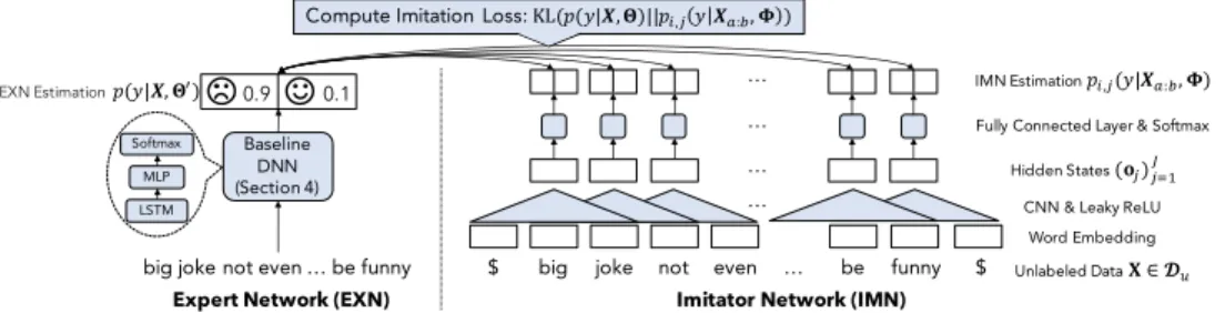
big joke not even … be funny Expert Network (EXN)

$ big joke not even … be funny $

…

Imitator Network (IMN)

CNN & Leaky ReLU Word Embedding Fully Connected Layer & Softmax

Hidden States(𝐨_#)_#%&^' IMN Estimation 𝑝_*,#(𝑦|𝑿_/:1, 𝚽)

…

…

…

Unlabeled Data𝐗 ∈ 𝓓6 EXN Estimation𝑝(𝑦|𝑿, 𝚯⁸)

MLP Softmax

LSTM

Compute Imitation Loss: KL(𝑝(𝑦|𝑿, 𝚯)||𝑝*,#𝑦 𝑿/:1, 𝚽 )

Figure 2: Overview of the 1st IMN (c

= 1). The IMN must predict the label estimation of the EXN from a limited amount of information. $ denotes a special token used to pad the input (a zero vector).

the core concept with the mixture-of-experts technique (MoE) [13, 14]. The difference is that MoE considers a mixture of several EXN s, whereas MEIN generates a mixture from a single EXN and a set of IMN s. In addition, one can interpret MEIN as a variant of the ensemble, bagging, voting, or boosting technique since the EXN and the IMN s jointly make a prediction. Moreover, we train each IMN by minimizing the KL-divergence between the EXN and the IMN through unlabeled data. This process can be seen as a form of “knowledge distillation” [15, 16]. We utilize these methodologies and formulate the framework as described below.

5.2 Network Architecture

Let σ( · ) be the sigmoid function defined as σ(λ) = (1 + exp( − λ))

. Φ denotes a set of trainable parameters of the IMN s and I denotes the number of IMN s.

Then, the EXN combined with a set of IMN s models the following (conditional) probability:

p(y | X , Θ, Φ, Λ) = exp(z

)

∑

y^′∈Y

exp(z

) , (5) where z

= z

+

∑

i=1

σ(λ

)α

[y]. (6)

λ

is a scalar parameter that controls the contribution of logit α

of the i-th IMN

and Λ is defined as Λ = { λ

, . . . , λ

} . Here, logit α

represents an estimated

label distribution, which we assume to be a feature. Note that the first term of

Equation 6 is the baseline DNN logit z

= w

s + b

(Equation 1). In addition, if we set σ(λ

) = 0 for all i, then Equation 5 becomes identical to Equation 2 regardless of the value of Φ.

c

denotes the window size of the i-th IMN . Given an input X and the i-th IMN , we create J inputs with a sliding window of size c

. Then the IMN predicts the EXN for each input and generates J predictions as a result. We compute the i-th imitator logit α

by taking the average of these predictions. Specifically, α

is defined as

α

= log ( 1

J

∑

j=1

p

(y | X

, Φ) )

, (7)

where a = j − c

and b = j + c

.

Here, a is a scalar index that represents the beginning of the window. Similarly, b represents the last index of the window.

5.3 Definition of IMNs

Note that the architecture of the IMN used to model Equation 7 is essentially ar- bitrary. In this research, we adopt a single-layer CNN for modeling p

(y | X

, Φ).

This is because a CNN has high computational efficiency [24], which is essential for our primary focus: scalability with the amount of unlabeled data.

Figure 2 gives an overview of the architecture of the IMN . First, the IMN takes a sequence of word embeddings of input X and computes a sequence of hidden states (o

)

by applying a one-dimensional convolution [25] and leaky ReLU nonlinearity [26]. We ensure that J is always equal to T . To achieve this, we pad the beginning and the end of the input X with zero vectors 0 ∈ R

, where |V

| denotes the vocabulary size of the IMN .

As explained in Section 5.2, each IMN has a predetermined and fixed window size c

. One can choose an arbitrary window size for the i-th IMN . Here, we define c

as c

= i for simplicity. For example, as shown in Figure 2, the 1st IMN (i = 1) has a window size of c

= 1. Such a network imitates the estimation of the EXN from three consecutive tokens.

Then the i-th IMN estimates the probability p

(y | X , Φ) from each hidden

Algorithm 1: Training framework of MEIN Data: Labeled data D

and unlabeled data D

Result: Trained set of parameters Θ, b Φ, b Λ b

1

Θ

← arg min

Θ

{ L

(Θ |D

) } ▷

2

Φ b ← arg min

Φ

{ L

(Φ | Θ

, D

) } ▷

Θ, b Λ b ← arg min

Θ,Λ

{ L

(Θ, Λ | Φ, b D

) } ▷

state o

as

p

(y | X

, Φ) = exp(w

o

+ b

)

∑

y^′∈Y

exp(w

o

+ b

) , (8) where w

∈ R

is the weight vector of the i-th IMN and b

is the scalar bias term of class y. N denotes the CNN kernel size.

5.4 Training Framework

First, we define the imitation loss of each IMN as the KL-divergence between the estimations of the label distributions of the EXN and the IMN given (unlabeled) data X, namely, KL(p(y | X , Θ) || p

(y | X

, Φ)). Note that this imitation loss is defined for an input with the sliding window X

. Thus, this definition effectively accomplishes the concept, i.e., the IMN making a prediction p

(y | X

, Φ) from only a limited view of the given input X

.

Next, our objective is to estimate the set of optimal parameters by minimizing the negative log-likelihood of Equation 5 while also minimizing the total imitation losses for all IMN s as biases of the network. Therefore, we jointly solve the following two minimization problems for the parameter estimation of MEIN :

Θ, b Λ b = arg min

Θ,Λ

{ L

(Θ, Λ | Φ, b D

) } (9) Φ b = arg min

Φ

{ L

(Φ | Θ

, D

) } . (10)

As described in Equations 9 and 10, we update the different sets of parameters

depending on the labeled/unlabeled training data. Specifically, we use the labeled

training data (X , y) ∈ D

to update the set of parameters in the EXN , Θ, and the set of mixture parameters of the IMN s, Λ. In addition, we use the unlabeled training data X ∈ D

to update the parameters of the IMN s, Φ.

To ensure an efficient training procedure, the training framework of MEIN consists of three consecutive steps (Algorithm 1). First, we perform standard supervised learning to obtain Θ

using labeled training data while keeping λ

=

−∞ unchanged for all i during the training process to ensure that σ(λ

) = 0 in Equation 6. Note that this optimization step is essentially equivalent to that of the baseline DNN (Equation 4).

Second, we estimate the set of IMN parameters Φ by solving the minimization problem in Equation 10 with the following loss function:

L

(Φ | Θ

, D

) = 1

|D

|

∑

X∈Du

∑

i=1

∑

j=1

KL(p || p

), (11) KL(p || p

) = − ∑

y∈Y

p(y | X , Θ

) log (

p

(y | X

, Φ) )

+ const, (12)

where KL(p || p

) is a shorthand notation of the imitation loss KL(p(y | X , Θ) || p

(y | X

, Φ)) and const is a constant term that is independent of Φ.

Finally, we estimate Θ and Λ by solving the minimization problem in Equa- tion 9 with the following loss function:

L

(Θ, Λ | Φ, b D

) = − 1

|D

|

∑

(X,y)∈D^s

log (

p(y | X , Θ, Φ,Λ) b )

. (13)

Task Dataset Classes Train Dev Test Unlabeled

SEC

Elec 2 22,500 2,500 25,000 200,000

IMDB 2 21,246 3,754 25,000 50,000

Rotten 2 8,636 960 1,066 7,911,684

CAC RCV1 55 14,007 1,557 49,838 668,640

Table 1: Summary of datasets. Each value represents the number of instances contained in each dataset.

6 Experiments

To investigate the effectiveness of MEIN , we conducted experiments on two text classification tasks: (1) a sentiment classification (SEC) task and (2) a category classification (CAC) task.

6.1 Datasets

For SEC, we selected the following widely used benchmark datasets: IMDB [27], Elec [28], and Rotten Tomatoes (Rotten) [29]. For the Rotten dataset, we used the Amazon Reviews dataset [30] as unlabeled data, following previous stud- ies [8, 1, 2]. For CAC, we used the RCV1 dataset [31]. Table 1 summarizes the characteristics of each dataset

.

6.2 Baseline DNNs

In order to investigate the effectiveness of the MEIN framework, we combined the IMN with following three distinct EXN s and evaluated their performance:

• LSTM : This is the baseline DNN (LSTM with MLP) described in Section 4.

• LM-LSTM : Following Dai and Le [8], we initialized the embedding layer and the LSTM with a pre-trained RNN-based language model (LM) [33].

2DBpedia [32] is another widely adopted CAC dataset. We did not use this dataset in our experiment because it does not contain unlabeled data.

We trained the language model using the labeled training data and un- labeled data of each dataset. Several previous studies have adopted this network as a baseline [1, 2].

• ADV-LM-LSTM : Adversarial training (ADV) [34] adds small perturba- tions to the input and makes the network robust against noise. Miyato et al. [1] applied ADV to LM-LSTM for a text classification. We used the reimplementation of their network.

Note that these three EXN s have an identical network architecture, as described in Section 4. The only difference is in the initialization or optimization strategy of the network parameters.

To the best of our knowledge, ADV-LM-LSTM provides a performance com- petitive with the current best result for the configuration of supervised learning (using labeled training data only). Thus, if the IMN can improve the perfor- mance of a strong baseline, the results will strongly indicate the effectiveness of our method.

6.3 Network Configurations

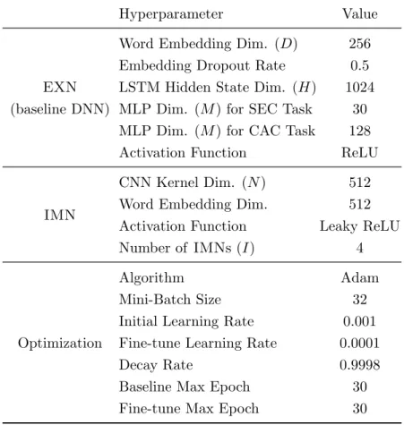
Table 2 summarizes the hyperparameters and network configurations of our ex- periments. We carefully selected the settings commonly used in the previous studies [8, 1, 2].

We used a different set of vocabulary for the EXN and the IMN s. We created the EXN vocabulary V by following the previous studies [8, 1, 2], i.e., we removed the tokens that appear only once in the whole dataset. We created the IMN vocabulary V

by byte pair encoding (BPE) [35]

. The BPE merge operations are jointly learned from the labeled training data and unlabeled data of each dataset.

We set the number of BPE merge operations to 20,000.

Hyperparameter Value

EXN (baseline DNN)

Word Embedding Dim. (D) 256

Embedding Dropout Rate 0.5

LSTM Hidden State Dim. (H) 1024

MLP Dim. (M ) for SEC Task 30

MLP Dim. (M ) for CAC Task 128

Activation Function ReLU

IMN

CNN Kernel Dim. (N ) 512

Word Embedding Dim. 512

Activation Function Leaky ReLU

Number of IMNs (I ) 4

Optimization

Algorithm Adam

Mini-Batch Size 32

Initial Learning Rate 0.001

Fine-tune Learning Rate 0.0001

Decay Rate 0.9998

Baseline Max Epoch 30

Fine-tune Max Epoch 30

Table 2: Summary of hyperparameters

6.4 Results

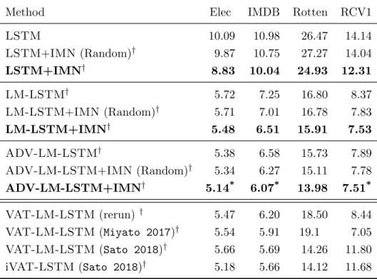
Table 3 summarizes the results on all benchmark datasets, where the evaluation metric is the error rate. Therefore, a lower value indicates better performance.

Here, all the reported results are the average of five distinct trials using five different random seeds. Moreover, for each trial, we automatically selected the best network in terms of the performance on the validation set among the net- works obtained at every epoch. For comparison, we also performed experiments on training baseline DNNs ( LSTM , LM-LSTM , and ADV-LM-LSTM ) with incorporating random vectors as the replacement of IMN s, which is denoted as

“+ IMN (Random)”. Moreover, we present the published results of VAT-LM-

3We used sentencepiece [36] (https://github.com/google/sentencepiece) for the BPE operations.

Method Elec IMDB Rotten RCV1

LSTM 10.09 10.98 26.47 14.14

LSTM + IMN (Random)

9.87 10.75 27.27 14.04

LSTM+IMN

8.83 10.04 24.93 12.31

LM-LSTM

5.72 7.25 16.80 8.37

LM-LSTM + IMN (Random)

5.71 7.01 16.78 7.83 LM-LSTM+IMN

5.48 6.51 15.91 7.53

ADV-LM-LSTM

5.38 6.58 15.73 7.89

ADV-LM-LSTM + IMN (Random)

5.34 6.27 15.11 7.78 ADV-LM-LSTM+IMN

5.14

6.07

13.98 7.51

VAT-LM-LSTM (rerun)

5.47 6.20 18.50 8.44 VAT-LM-LSTM (Miyato 2017)

5.54 5.91 19.1 7.05 VAT-LM-LSTM (Sato 2018)

5.66 5.69 14.26 11.80

iVAT-LSTM (Sato 2018)

5.18 5.66 14.12 11.68

Table 3: Test performance (error rate (%)) on each dataset. A lower error rate indicates better performance. Models using the unlabeled data are marked with † . Results marked with

are statistically significant compared with ADV- LM-LSTM . Miyato 2017: the result reported by Miyato et al. [1]. Sato 2018:

the result reported by Sato et al. [2].

LSTM [1] and i VAT-LSTM [2] in the bottom three rows of Table 3, which are the current state-of-the-art networks that adopt unlabeled data. For VAT- LM-LSTM , we also report the result of the reimplemented network, denoted as

“ VAT-LM-LSTM (rerun)”.

As shown in Table 3, incorporating the IMN s consistently improved the perfor- mance of all baseline DNNs across all benchmark datasets. Note that the source of these improvements is not the extra set of parameters Λ but the outputs of the IMN s. We can confirm this fact by comparing the results of IMN s, “+ IMN ”, with those of random vectors, “+ IMN (Random)”, since the difference between these two settings is the incorporation of IMN s or random vectors.

The most noteworthy observation about MEIN is that the amount of the

improvement upon incorporating the IMN is nearly consistent, regardless of the

performance of the base EXN . For example, Table 3 shows that the IMN reduced the error rates of LSTM , LM-LSTM , and ADV-LM-LSTM by 1.54%, 0.89%, and 1.22%, respectively, for the Rotten dataset. From these observations, the IMN has the potential to further improve the performance of much stronger EXN s developed in the future.

We also remark that our best configuration, ADV-LM-LSTM + IMN , outper- formed VAT-LM-LSTM (rerun) on all datasets

. In addition, the best config- uration outperformed the current best published results on the Elec and Rotten datasets, establishing new state-of-the-art results.

As a comparison with the current strongest SSL method, we combined the IMN with the current state-of-the-art VAT method, namely, VAT-LM-LSTM + IMN . In the Elec dataset, the IMN improved the error rate from 5.47% to 5.16%. This result indicates that the IMN and VAT have a complementary relationship. Note that utilizing VAT is challenging in terms of the scalability with the amount of unlabeled data. However, if sufficient computing resources exist, then VAT and the IMN can be used together to achieve even higher performance.

4The performance of ourVAT-LM-LSTM(rerun) is lower than the performances reported by Miyato et al. [1] except for the Elec and Rotten datasets. Through extensive trials to reproduce their results, we found that the hyperparameter of the RNN language model is extremely important in determining the final performance; therefore, the strict reproduction of the published results is significantly difficult. In fact, a similar difficulty can be observed in Table 3, whereVAT-LM-LSTM (Sato 2018) has lower performance than VAT-LM-LSTM (Miyato 2017) on the Elec and RCV1 datasets. Thus, we believe thatVAT-LM-LSTM(rerun) is the most reliable result for the comparison.

7 Analysis

7.1 More Data, Better Performance Property

We investigated whether the MEIN framework has the more data, better per- formance property for unlabeled data. Ideally, MEIN should achieve better performance by increasing the amount of unlabeled data. Thus, we evaluated the performance while changing the amount of unlabeled data used to train the IMN .

We selected the Elec and RCV1 datasets as the focus of this analysis. We created the following subsamples of the unlabeled data for each dataset: { 5K, 20K, 50K, 100K, Full Data } for Elec and { 5K, 50K, 250K, 500K, Full Data } for RCV1. In addition, for the Elec dataset, we sampled extra unlabeled data from the electronics section of the Amazon Reviews dataset [30] and constructed { 2M, 4M, 6M } unlabeled data

. For each (sub)sample, we trained ADV-LM- LSTM + IMN as explained in Section 6.

Figures 3a and 3b demonstrate that increasing the amount of unlabeled data improved the performance of the EXN . It is noteworthy that in Figure 3a, ADV- LM-LSTM + IMN trained with 6M data achieved an error rate of 5.06%, outper- forming the best result in Table 3 (5.14%). These results explicitly demonstrate the more data, better performance property of the MEIN framework. We also report that the training process on the largest amount of unlabeled data (6M) only took approximately a day.

7.2 Scalability with Amount of Unlabeled Data

The primary focus of the MEIN framework is its scalability with the amount of unlabeled data. Thus, in this section, we compare the computational speed of the IMN s with that of the base EXN . We also compare the IMN s with the state- of-the-art SSL method, VAT-LM-LSTM , and discuss their scalability. Here, we focus on the computation in the training phase of the network, where the network

5We discarded instances from the unlabeled data when the non stop-words overlap with instances in the Elec test set. Thus, the unlabeled data and the Elec test set had no instances in common.

10² 10³ 10⁴ 10⁵ 10⁶ Amount of Unlabeled Data (|Du|) 5.2

5.4 5.6

ErrorRate(%)

Baseline (ADV-LM-LSTM)

(a) Elec

10² 10³ 10⁴ 10⁵ 10⁶ Amount of Unlabeled Data (|Du|) 7.5

7.6 7.7 7.8 7.9

ErrorRate(%)

Baseline (ADV-LM-LSTM)

(b) RCV1

Figure 3: Error rate (%) at different amounts of unlabeled data. The x-axis is in log-scale. A lower error rate indicates better performance. The dashed horizontal line represents the performance of the base EXN ( ADV-LM-LSTM ).

Method Tokens/sec Relative Speed

LM-LSTM 41,914 -

ADV-LM-LSTM 13,791 0.33x

VAT-LM-LSTM 9,602 0.23x

IMN (c

= 1) 555,613 13.26x

IMN (c

= 1, 2) 236,065 5.63x

IMN (c

= 1, 2, 3) 122,076 2.91x

IMN (c

= 1, 2, 3, 4) 75,393 1.80x

Table 4: Number of tokens processed per second during the training processes both forward and backward computations.

We measured the number of tokens that each network processes per second. We

used identical hardware for each measurement, namely, a single NVIDIA Tesla

V100 GPU. We used the cuDNN implementation for the LSTM cell since it is

highly optimized and substantially faster than the naive implementation [37].

Base A B C D 4.0

4.5 5.0 5.5 6.0

Erro r Rate (%)

Elec

Base A B C D

4 5 6 7 8

Erro r Rate (%)

6.23 6.23 6.15 6.07

IMDB

Base A B C D

10 12 14 16

Erro r Rate (%)

15.73

14.68 14.53 14.51 13.98

Rotten Tomatoes

Base A B C D

5 6 7 8 9

Erro r Rate (%)

RCV1

Figure 4: Effect of the IMN with different window sizes c

on the final error rate (%) of ADV-LM-LSTM . A lower error rate indicates better per- formance. Base: EXN ( ADV-LM-LSTM ) without the IMN , A: c

= 1, B:

c

= 1, 2, C: c

= 1, 2, 3, D: c

= 1, 2, 3, 4.

Table 4 summarizes the results. The table shows that even the slowest IMN

(c

= 1, 2, 3, 4) was 1.8 times faster than the optimized cuDNN LSTM network

and eight times faster than VAT-LM-LSTM . This indicates that it is possible

to use an even larger amount of unlabeled data in a practical time to further

improve the performance of the EXN . In addition, note that each IMN can be

trained in parallel. Thus, if multiple GPUs are available, the training can be

carried out much faster than reported in Table 4.

7.3 Effect of Window Size of the IMN

In this section, we investigate the effectiveness of combining IMN s with different

window sizes c

on the final performance of the EXN . Figure 4 summarizes the

results across all datasets. The figure shows that integrating an IMN with a

greater window size consistently reduced the error rate, and the IMN with the

greatest window size (D: c

= 1, 2, 3, 4) achieved the best performance. This

observation implies that the context, which is captured by a greater window size,

contributes to the performance.

Window Size Error Rate (%)

c

= 1, 2, 3, 4 5.14

c

= 2, 3, 4 5.18

c

= 3, 4 5.26

c

= 4 5.23

Table 5: Effect of removing IMN s with smaller window sizes on the error rate (%) of ADV-LM-LSTM on the Elec dataset. A lower error rate indicates better performance.

8 Discussion

8.1 Variations of the IMN

In this section, we discuss two possible variations of the IMN to better understand its effectiveness in the MEIN framework.

8.1.1 Incorporating IMN with Greater Window Size

As discussed in Section 7.3, Figure 4 demonstrates that increasing the window size of the IMN consistently improves the performance. From this observation, one may hypothesize that integrating an IMN with an even greater window size will be beneficial. Thus, we carried out an experiment with such a configuration, i.e., c

= 1, 2, 3, 4, 5, and found that the hypothesis is valid. For example, the error rates of ADV-LM-LSTM + IMN (c

= 1, 2, 3, 4, 5) were 5.12% and 6.00%

for Elec and IMDB, respectively, which are better than the values reported in Table 3.

However, we found that a large window size has a major drawback; the training

of IMN s becomes significantly slower. This undesirable property must be avoided

as our primary focus is the scalability with the amount of unlabeled data. Thus,

we do not report these values as the main results of the experiment in Table 3.

8.1.2 Removing IMNs with Smaller Window Sizes

We also investigated the effectiveness of utilizing IMN s with smaller window size in addition to the larger window sizes. Table 5 gives the results of this investigation, and we can see that combining IMN s with smaller window sizes works better than incorporating a single IMN with the greatest window size.

8.2 Stronger Baseline DNN

In this section, we discuss the results of two attempts to improve the performance of baseline DNNs.

8.2.1 Increasing Number of Parameters

The most straightforward means of improving the performance of baseline DNNs is to increase the number of parameters. Thus, we doubled the word embedding dimension and trained ADV-LM-LSTM , namely, the ADV-LM-LSTM -Large model. This model has approximately the same number of parameters as the ADV-LM-LSTM + IMN . However, the performance did not improve from that of the original ADV-LM-LSTM . Specifically, the error rate degraded by 0.08 points for the IMDB dataset and was unchanged for the Elec dataset.

8.2.2 Combining ELMo

ELMo [10] is one of the strongest SSL approaches in the research field. Thus, we conducted an experiment with a baseline that utilizes ELMo. Specifically, we combined LSTM with the ELMo embeddings, namely, ELMo-LSTM

. The error rate of this network on the IMDB test set was 8.67%, which is worse than that of LM-LSTM reported in Table 3. This result suggests that, at least in this task setting, pre-training the RNN language model for initialization is more effective than using the ELMo embeddings.

6We used the implementation available in AllenNLP [38].

9 Conclusion

In this paper, we proposed a novel method for SSL, which we named Mixture of Expert/Imitator Networks ( MEIN ). The MEIN framework consists of a baseline DNN, i.e., an EXN , and several auxiliary networks, IMN s. The unique property of our method is that the IMN s learn to “imitate” the estimated label distribution of the EXN over the unlabeled data with only a limited view of the given input. In this way, the IMN s effectively learn a set of features that potentially contributes to improving the classification performance of the EXN .

Experiments on text classification datasets demonstrated that the MEIN frame-

work consistently improved the performance of three distinct settings of the EXN .

We also trained the IMN s with extra large-scale unlabeled data and achieved a

new state-of-the-art result. This result indicates that our method has the more

data, better performance property. Furthermore, our method operates eight times

faster than the current strongest SSL method (VAT), and thus, it has promising

scalability to the amount of unlabeled data.

Acknowledgements

I am deeply grateful to Dr. Kentaro Inui and Dr. Jun Suzuki for able guidance

and generous support. I would like to show my greatest appreciation to Dr. Sho

Takase for insightful comments and constructive suggestions. Discussions with

my academic colleagues in our laboratory have been quite illuminating.

References

[1] Takeru Miyato, Andrew M Dai, and Ian Goodfellow. Adversarial Training Methods For Semi-Supervised Text Classification. In Proceedings of the 5th International Conference on Learning Representations (ICLR 2017), 2017.

[2] Motoki Sato, Jun Suzuki, Hiroyuki Shindo, and Yuji Matsumoto. Inter- pretable Adversarial Perturbation in Input Embedding Space for Text. In Proceedings of the 27th International Joint Conference on Artificial Intelli- gence and the 23rd European Conference on Artificial Intelligence (IJCAI- ECAI 2018), pages 4323–4330, 2018.

[3] Kaiming He, Xiangyu Zhang, Shaoqing Ren, and Jian Sun. Deep Residual Learning for Image Recognition. In 2016 IEEE Conference on Computer Vision and Pattern Recognition (CVPR 2016), pages 770–778, 2016.

[4] Dario Amodei, Sundaram Ananthanarayanan, Rishita Anubhai, Jingliang Bai, Eric Battenberg, Carl Case, Jared Casper, Bryan Catanzaro, Qiang Cheng, Guoliang Chen, et al. Deep Speech 2: End-to-End Speech Recog- nition in English and Mandarin. In Proceedings of the 33rd International Conference on Machine Learning (ICML 2016), pages 173–182, 2016.

[5] Yonghui Wu, Mike Schuster, Zhifeng Chen, Quoc V Le, Mohammad Norouzi, Wolfgang Macherey, Maxim Krikun, Yuan Cao, Qin Gao, Klaus Macherey, et al. Google’s Neural Machine Translation System: Bridging the Gap be- tween Human and Machine Translation. arXiv preprint arXiv:1609.08144, 2016.

[6] Jia Deng, Wei Dong, Richard Socher, Li-Jia Li, Kai Li, and Li Fei-Fei. Im- ageNet: A Large-Scale Hierarchical Image Database. In 2009 IEEE Con- ference on Computer Vision and Pattern Recognition (CVPR 2009), pages 248–255, 2009.

[7] Tomas Mikolov, Ilya Sutskever, Kai Chen, Greg S Corrado, and Jeff Dean.

Distributed Representations of Words and Phrases and their Compositional-

ity. In Advances in Neural Information Processing Systems 26 (NIPS 2013),

pages 3111–3119, 2013.

[8] Andrew M Dai and Quoc V Le. Semi-supervised Sequence Learning. In Advances in Neural Information Processing Systems 28 (NIPS 2015), pages 3079–3087, 2015.

[9] Kevin Clark, Thang Luong, and Quoc V. Le. Cross-View Training for Semi- Supervised Learning. In Proceedings of the 6th International Conference on Learning Representations (ICLR 2018), 2018.

[10] Matthew Peters, Mark Neumann, Mohit Iyyer, Matt Gardner, Christopher Clark, Kenton Lee, and Luke Zettlemoyer. Deep Contextualized Word Rep- resentations. In Proceedings of the 2016 Conference of the North American Chapter of the Association for Computational Linguistics: Human Language Technologies (NAACL 2018), pages 2227–2237, 2018.

[11] Jeffrey Pennington, Richard Socher, and Christopher Manning. GloVe:

Global Vectors for Word Representation. In Proceedings of the 2014 Confer- ence on Empirical Methods in Natural Language Processing (EMNLP 2014), pages 1532–1543, 2014.

[12] Rafal Jozefowicz, Oriol Vinyals, Mike Schuster, Noam Shazeer, and Yonghui Wu. Exploring the Limits of Language Modeling. arXiv preprint arXiv:1602.02410, 2016.

[13] Robert A Jacobs, Michael I Jordan, Steven J Nowlan, and Geoffrey E Hinton.

Adaptive Mixtures of Local Experts. Neural Computation, 3(1):79–87, 1991.

[14] Noam Shazeer, Azalia Mirhoseini, Krzysztof Maziarz, Andy Davis, Quoc Le, Geoffrey Hinton, and Jeff Dean. Outrageously Large Neural Networks:

The Sparsely-Gated Mixture-of-Experts Layer. In Proceedings of the 5th International Conference on Learning Representations (ICLR 2017), 2017.

[15] Jimmy Ba and Rich Caruana. Do Deep Nets Really Need to be Deep? In Advances in Neural Information Processing Systems 27 (NIPS 2014), pages 2654–2662, 2014.

[16] Geoffrey Hinton, Oriol Vinyals, and Jeffrey Dean. Distilling the Knowledge

in a Neural Network. In NIPS Deep Learning and Representation Learning

Workshop, 2015.

[17] Bryan McCann, James Bradbury, Caiming Xiong, and Richard Socher.

Learned in Translation: Contextualized Word Vectors. In Advances in Neu- ral Information Processing Systems 30 (NIPS 2017), pages 6294–6305, 2017.

[18] Matthew Peters, Waleed Ammar, Chandra Bhagavatula, and Russell Power.

Semi-supervised Sequence Tagging with Bidirectional Language Models. In Proceedings of the 55th Annual Meeting of the Association for Computational Linguistics (ACL 2017), pages 1756–1765, 2017.

[19] Jun Suzuki and Hideki Isozaki. Semi-Supervised Sequential Labeling and Segmentation Using Giga-Word Scale Unlabeled Data. In Proceedings of the 46th Annual Meeting of the Association for Computational Linguistics (ACL 2008), pages 665–673, 2008.

[20] Ciprian Chelba, Tomas Mikolov, Mike Schuster, Qi Ge, Thorsten Brants, Phillipp Koehn, and Tony Robinson. One Billion Word Benchmark for Mea- suring Progress in Statistical Language Modeling. In INTERSPEECH, pages 2635–2639, 2014.

[21] Sepp Hochreiter and J¨ urgen Schmidhuber. Long Short-Term Memory. Neu- ral Computation, 9(8):1735–1780, 1997.

[22] Xavier Glorot, Antoine Bordes, and Yoshua Bengio. Deep Sparse Rectifier Neural Networks. In Proceedings of the Fourteenth International Conference on Artificial Intelligence and Statistics (AISTATS 2011), pages 315–323, 2011.

[23] Diederik Kingma and Jimmy Ba. Adam: A Method for Stochastic Opti- mization. In Proceedings of the 3rd International Conference on Learning Representations (ICLR 2015), 2015.

[24] Jonas Gehring, Michael Auli, David Grangier, Denis Yarats, and Yann N

Dauphin. Convolutional Sequence to Sequence Learning. In Proceedings of

the 34th International Conference on Machine Learning (ICML 2017), pages

1243–1252, 2017.

[25] Nal Kalchbrenner, Edward Grefenstette, and Phil Blunsom. A Convolutional Neural Network for Modelling Sentences. In Proceedings of the 52nd Annual Meeting of the Association for Computational Linguistics (ACL 2014), pages 655–665, 2014.

[26] Andrew L Maas, Awni Y Hannun, and Andrew Y Ng. Rectifier Nonlinearities Improve Neural Network Acoustic Models. In ICML Workshop on Deep Learning for Audio, Speech, and Language Processing, 2013.

[27] Andrew L. Maas, Raymond E. Daly, Peter T. Pham, Dan Huang, Andrew Y.

Ng, and Christopher Potts. Learning Word Vectors for Sentiment Analysis.

In Proceedings of the 49th Annual Meeting of the Association for Computa- tional Linguistics (ACL 2016), pages 142–150, 2011.

[28] Rie Johnson and Tong Zhang. Semi-supervised Convolutional Neural Net- works for Text Categorization via Region Embedding. In Advances in Neural Information Processing Systems 28 (NIPS 2015), pages 919–927, 2015.

[29] Bo Pang and Lillian Lee. Seeing Stars: Exploiting Class Relationships for Sentiment Categorization with Respect to Rating Scales. In Proceedings of the 43rd Annual Meeting of the Association for Computational Linguistics (ACL 2005), pages 115–124, 2005.

[30] Julian McAuley and Jure Leskovec. Hidden Factors and Hidden Topics:

Understanding Rating Dimensions with Review Text. In Proceedings of the 7th ACM conference on Recommender systems (RecSys 2013), pages 165–

172, 2013.

[31] David D. Lewis, Yiming Yang, Tony G. Rose, and Fan Li. RCV1: A New Benchmark Collection for Text Categorization Research. Journal of Machine Learning Research, 5:361–397, 2004.

[32] Jens Lehmann, Robert Isele, Max Jakob, Anja Jentzsch, Dimitris Kon-

tokostas, Pablo N Mendes, Sebastian Hellmann, Mohamed Morsey, Patrick

Van Kleef, S¨ oren Auer, et al. DBpedia–a large-scale, multilingual knowledge

base extracted from Wikipedia. Semantic Web, 6(2):167–195, 2015.