Finite Element Modelling of the Transduction Properties of Lead- Zirconate-Titanate Materials

Finite Element Modelling of the Transduction Properties of Lead- Zirconate-Titanate Materials

M.L.Lee

., W.K.Chiu

and N.Rajic

1- Department of Mechanical Engineering, Monash University, Clayton, Victoria 3800, Australia 2 - Defence Science and Technology Organisation, Platforms Sciences Laboratory, Air Vehicles Division, Fishermens Bend 3207, Victoria, Australia

The finite element (FE) modelling of Lead-Zirconate-Titanate (PZT) patches bonded onto aluminium plates for the purposes of exciting Lamb waves is investigated. Lamb wave propagation in plate-like structures is used as an important tool for non-destructive structural health monitoring. In particular this paper focuses on the PZT transduction process by modelling the patch as a 3D orthotropic material. Two main criteria were used to define successful modelling of the PZT patch to the aluminium plate. Firstly, the physical reaction of the PZT patch must conform to the constitutive relationships for piezoceramic materials.

Secondly, the patch must be shown to have successfully excited Lamb waves within the plate structure by satisfying the wave dispersion properties. It was found that the 3D orthotropic model satisfied both the above conditions. The adequacy of the 3D orthotropic model was also further substantiated by comparing the strength of the propagated waves with results experimentally measured by laser vibrometry.

Keywords: Modelling PZT Transduction, Constitutive Relations, Lamb Wave, Laser Vibrometry

1 Introduction

The use of ultrasonic guided waves in detecting defects in plate-like structures is well established. Some examples of earlier works include Alleyne’s seminal dissertation regarding The Non-destructive Testing of Plates using Ultrasonic Lamb Waves [1] and other important works such as [2, 3]. The feasibility of using piezoelectric materials, of which the PZT belongs, in order to generate Lamb waves was first demonstrated by Beard and Chang [4].

Furthermore, the use of Lamb waves have also been incorporated into non-destructive testing techniques such as ultrasonic lamb wave tomography and applied not only to isotropic metallic structures but also to composite plates and repair patches [5, 6]. With the increase in computational speeds and efficiencies over the last decade, many researchers are increasingly augmenting their experimental work with FE modelling and analysis. Traditionally, in order to study lamb wave propagation in plates by numerical methods, the wave excitation relied on applying point loads on the plate structure. For example, a symmetric wave mode would be excited by simultaneously pulling apart two nodes on the top and bottom surfaces of the plate.

Whilst effective in exciting the required symmetric Lamb mode, the point excitation method is not representative of the PZT transduction process. It is the intention of this paper to provide a simple and clear method by which correct Lamb wave propagation can be achieved in the FE environment by correctly modelling the transduction from the PZT material into an aluminium plate.

2 Constitutive Relationships: Piezo-ceramic Materials

The general constitutive equations of linear piezo-electric behaviour are described by two tensorial relationship equations. This paper is primarily concerned with the relationship between mechanical strain (S) and stress (T) as given by,

E

+

= (1)

where E is the electric field, the lower case s is the compliance tensor of the material which is measured at zero electric field stress and d is the piezo-electric coupling between the mechanical and electrical variables. Reference [7] explains that if the ceramic is free to expand, then the T tensor in equation (1) goes to zero leaving the mechanical strain S to be only the products of the applied electric field E and the piezo-electric coupling constant d.

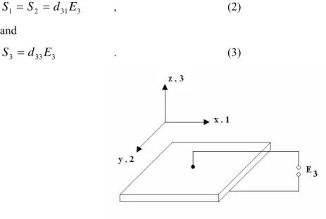
With respect to the directions as defined by figure 1, equation (1) then becomes the following condition as shown in equations (2) and (3) by which we define successful physical modelling of the PZT patch;

3 31 2

1

S d E

S = = , (2)

and

3 33

3

d E

S = . (3)

Figure 1. Reference Axis

That is, the FE model of the PZT patch is said to be physically representative of a real patch if equations (2) and (3) hold given that for a typical soft compound PZT material d

is (-1.75 E- 10 m/V) and d

is (3.75 E-10 m/V) [7].

3 PZT Material Properties

The PZT modelled in this study represents a special case of an orthotropic material in that it possesses a transverse plane which is isotropic. As such it is vitally important to correctly represent the material properties in the FE code. It is worth noting at this stage that certain commercial codes utilise slightly different convention in defining the shear stresses and as such care must be taken when characterising the material properties. The equation (4) shows the stiffness matrix necessary when modelling transversely isotropic materials;

⎪ ⎪

⎪ ⎪

⎭

⎪⎪

⎪ ⎪

⎬

⎫

⎪ ⎪

⎪ ⎪

⎩

⎪⎪

⎪ ⎪

⎨

⎧

zx yz xy zz yy xx

σ σ σ σ σ σ

=

⎥ ⎥

⎥ ⎥

⎥ ⎥

⎥ ⎥

⎦

⎤

⎢ ⎢

⎢ ⎢

⎢ ⎢

⎢ ⎢

⎣

⎡

66 55 44 33 23 22

13 12 11

0 0 0

0 0 0

0 0 0

0 0 0

C C C C C C

C C C

⎪ ⎪

⎪ ⎪

⎭

⎪⎪

⎪ ⎪

⎬

⎫

⎪ ⎪

⎪ ⎪

⎩

⎪⎪

⎪ ⎪

⎨

⎧

zx yz xy zz yy xx

γ γ γ ε ε ε

(4)

where σ is stress, τ is shear stress, ε is strain and γ is shear strain. Individual elements within the stiffness matrix are represented by,

symmetric

Δ

= −

3 1

31 13 11

1 E E

v

C v (5)

Δ

= +

3 1

13 31 13

12

E E

v v

C v (6)

Δ

= +

3 1

31 13 31

13

E E

v v

C v (7)

Δ

= −

1 2 33 13

1 E

C v (8)

) 1

(

2

2 1

44

v v

E C E

= + (9)

) 1

(

2

3 2

55

v v

E C E

= + (10)

) 1

(

2

1 3

66

v v

E C E

= + (11)

3 2 1

31 13 1

1

)( 1 2 )

1 (

E E

v v v v − −

= +

Δ (12)

11

22

C

C = (13) C

= C

(14)

The symbol v is the poisson’s ratio and E is the young’s modulus of elasticity. The subscript convention used is such that v

represents the poisson’s ratio in i due to an action in j. In this study, the plane of isotropy is in the x-y plane such that; E

and E

is equal to 7.14E+10 Pa and v

is equal to v

at 0.3. Perpendicular to the plane of isotropy we define E

as 5.26E+10 Pa and an initial assumption was made that v

was equal to 0.3 and subsequently given that,

3 31 1 13

E v E

v = (15)

then, v

is 0.221. Also, since the plane of isotropy is x-y, then E

= E

and v

= v

. 4 Lamb Wave Dispersion Curves

In section 2 it was described that in order for the modelled PZT patch to be physically representative of a real patch; its expansion-contraction behaviour under loading must conform to the constitutive relationships given by equations (2) and (3). Upon successfully modelling the mechanical action of the PZT patch under loading, the next step is to ensure the excitation is correctly transducted into the plate on which the patch is bonded. To confirm that Lamb waves are correctly excited by the PZT mechanical action, a series of equi-spaced nodes along the top surface of the modelled aluminium plate were probed to obtain nodal displacement time histories. A 2D-FFT technique was then used in order to decompose the received signals into its frequency and wave number domains. Excited Lamb wave modes should be evident by comparing against theoretically derived wave number vs. frequency dispersion curves.

5 PZT Patch FE Model

A 0.01m x 0.01m x 0.001m (40 x 40 x 4 elements) PZT patch model was generated using

regular quad type elements. The patch was constrained along the top and bottom surfaces to

only allow translation in the z direction. This means of constraining forces the patch to

undergo expansion along its side walls for an applied compressive force on the top and

bottom surface. Previously it was found that without the mentioned constraint, the edges

along the top and bottom surfaces of the patch showed a propensity to “fold” over under

compressive force application and thus did not represent a realistic deformation of a PZT

Under an arbitrary compressive load and given that E

and E

are constants; the poisson’s ratio v

was systematically varied until the calculated stiffness matrix for the modelled PZT material allowed the modelled patch to compress and expand according to the relations given in equations (2) and (3). That is,

33 31 3 1

d d S

S = (16)

where S

is equal to S

.

Figure 2. 3D PZT Patch Model

For the PZT modelled in this study the values of the elastic constants E

and E

are 7.14 E+10 Pa and 5.26 E+10 Pa. The constant v

was initially set to 0.3. Now given d

and d

in section 2, then the theoretical mechanical expansion-compression ratio for this PZT should be 0.467 according to equation (13). It was found that with the poisson’s ratio v

= 0.32, the expansion-compression ratio as obtained by the model expansion in the x or y-axis and its compression in the z-axis was 0.460. This result is within 1.5% of the theoretical ratio. It was not yet possible to transplant the PZT patch model in its current state directly onto the complete PZT-adhesive-Aluminium plate model. The current PZT patch mesh must be made coarser to match the meshing regime defined for the plate in order to be computationally efficient. The above FE experiment was then repeated for a model with the same dimensions but coarser mesh (10 x 10 x 2 elements). It was found that the expansion-compression ratio for coarser mesh then become 0.430. This result is within 8% of the theoretical result and sufficient such that the coarser patch model could then be directly transplanted onto the complete plate model.

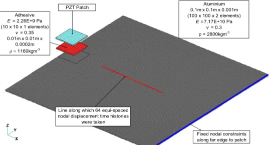
6 PZT-Adhesive-Aluminium Model

The complete 3D model comprises of three layers being the PZT patch, the adhesive and the aluminium plate. Figure 3 shows the layers and their respective material properties. The PZT patch itself was constrained as given in figure 2 with a compressive impulse excitation applied to the top and bottom surface. The impulse excitation was of duration 4.6E-6 s thus giving sufficient impulse energy to excite up to 600 kHz. Although impulse excitation excites a band of frequencies, decomposition into the wave number and frequency domains should see the signals separated into their respective symmetric and anti-symmetric Lamb modes. As introduced in section 4, in order to utilise the 2D-FFT technique for wave number – frequency domain decomposition, time history data must be gathered along a line of equi-spaced nodes.

The figure 3 also indicates the line along which nodal displacement time histories were

obtained. The derivation of the analytical curves against which the decomposed received

signals are compared against can be found in [1, 8].

PZT Patch Adhesive

E = 2.26E+9 Pa (10 x 10 x 1 elements)

v = 0.35 0.01m x 0.01m x

0.0002m ρ = 1160kgm^-3

Aluminium 0.1m x 0.1m x 0.001m (100 x 100 x 2 elements)

E =7.17E+10 Pa v = 0.3 ρ = 2800kgm^-3

Line along which 64 equi-spaced nodal displacement time histories

were taken

Fixed nodal constraints along far edge to patch

Figure 3. Complete FE Model of PZT Patch Bonded onto Aluminium Plate

a)

0 0.2 0.4 0.6 0.8 1 1.2 1.4 1.6 1.8 2

0 500 1000 1500 2000 2500 3000

Frequency(MHz)

Wavenumber(rad/m)

2-D FFT Symmetric Modes Anti-symmetric Modes

0.5 1 1.5 2 2.5 3 3.5 4 4.5 5 x 10^-9

b)

0.2 0.4 0.6 0.8 1 1.2 1.4 1.6 1.8 2

0 500 1000 1500 2000 2500

Frequency(MHz)

W a ve nu m b er (r a d/ m )

2-D FFT Symmetric Modes Anti-symmetric Modes

2 4 6 8 10 12 14 16 x 1018 ^-9

Figure 4a. Decomposition of Waves in the Frequency-Wave number domain vs.

Analytical dispersion curves (Out-of-plane)

Figure 4a shows the wave number – frequency domain decomposition of the out-of-plane (z- direction) motion along the 64 nodes. It can be seen that the presented method of PZT patch modelling and excitation was successful in exciting the zero-th anti-symmetric Lamb mode (A0) in the modelled plate. It should be noted that a dual frequency and wave number filter was applied as a post-process to allow frequencies between 150 kHz to 1.5MHz to and wave numbers above 100 to pass. A dominant A0 mode can be observed at around 500 kHz. Figure 4b shows the dispersion plot of the same scenario but using only the latter 256 time points of the last 32 spatial nodes for analysis. This scenario did not require any filtering and it is clear that the A0 mode is evidently dominant at around 500 kHz.

7 Laser Vibrometry Experiments

Further to the 2D-FFT technique, a laser vibrometry experiment was also performed to verify that the model realisation of the Lamb waves were realistic. A PZT patch of similar dimensions to that modelled was bonded onto a 0.1m x 0.1m x 0.001m aluminium plate.

Although the FE model had a cantilever style constraint along the far edge to the PZT patch, this physical model simply clipped the plate at 2 corners. A HP 33120A signal generator was used to deliver an impulse excitation into the PZT patch of similar duration to the modelled excitation. The out-of-plane displacement of a series of points at a constant radius of 25mm from the PZT patch was measured by use of a Polytec OFV505 laser vibrometer. Similarly, the out-of-plane displacements at the equivalent locations were also obtained from the FE model. Figure 5 shows part of the experimental set up and a schematic of the positions at which the out-of-plane displacements were read around the PZT patch.

25mm

Figure 5. Polytec OFV505 Laser vibrometer measuring out-of-plane displacements on aluminium plate

Firstly, comparing the points directly above the PZT patch, it can be seen that the raw

frequency response of both the FE and the experimental case share common features in terms

of the modes excited. This is shown in figure 6. A time domain comparison also shows that

the arriving wave packet in both the experimental and FE case show notable similarity (figure

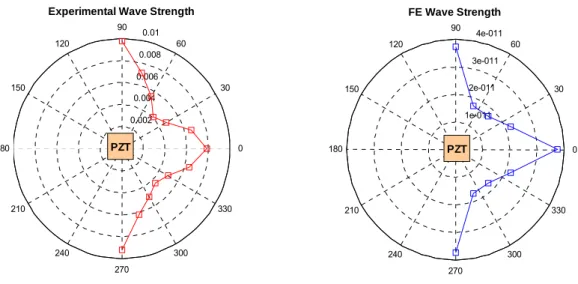
7). The wave strength at a given location is defined as the root mean square (RMS) value of

the out-of-plane displacements. Thus the wave strengths of the FE and experimental scenarios

can be compared by calculating the RMS values of those selected points at a constant radius

around the PZT patch in both the FE and experimental cases. When a low time window was

applied to the response data at points around the PZT the shape of the wave strength plot

between the FE and experimental cases showed good agreement. Figure 8 show typically the

response data at 2 corresponding points on the experimental case and the FE model. Whilst

figure 9 show the similarity in wave strength at a constant radii around the PZT patch when

only the low time windowed data was considered.

0 1 2 3 4 5 6 7 8 x 10⁵ 0

2 4 6 8 10 12 14 16 18

Frequency (Hz)

Magnitude

0 1 2 3 4 5 6 7 8

x 10⁵ 0

0.5 1

x 10^-8

Frequency (Hz)

Magnitude

Experimental Magnitude

Spectra FE Magnitude Spectra

Figure 6. Frequency domain comparison of typical out-of-plane displacement signals from FE and Experimental setup

Figure 7. Experimental vs. FE Time history comparison of input impulse and response of aluminium at 25mm from PZT patch centre

0 0.5 1 1.5 2 2.5 3 3.5 4 4.5

x 10^-5 -1.5

-1 -0.5 0 0.5 1 1.5

2x 10^-10

Time (s)

Magnitude (m)

Low Time Windowed FE Response

0.5 1 1.5 2 2.5 3 3.5 4 4.5

x 10^-5 -0.04

-0.03 -0.02 -0.01 0 0.01 0.02 0.03 0.04 0.05 0.06

Time (s)

Magnitude (V)

Low Time Windowed Experimental Response

Figure 8. Low time windowed response comparison

0.002 0.004

0.006 0.008 0.01

30

210

60

240

90

270 120

300 150

330

180 0

Experimental Wave Strength

1e-011 2e-011

3e-011 4e-011

30

210

60

240

90

270 120

300 150

330

180 0

FE Wave Strength

PZT PZT

Figure 9. Wave strength comparison between experimental and FE cases

8 Conclusions

The transduction process is a complex problem and the presented methodology presents a simple method by which the PZT when properly modelled and constrained can be excited such that its mechanical action obeys the piezoceramic constitutive relations. Subsequently Lamb waves were successfully excited through the modelled aluminium plate. This paper successfully presents an alternative to Lamb wave excitation modelling compared to the traditional point excitation method. It also improves on the traditional method by showing that above and beyond Lamb wave generation this current methodology also successfully mimics the physical wave propagation characteristic in terms of wave strength.

Acknowledgements

The authors would like to acknowledge the help of Mr Long Kim Goh for aiding in the preparation of the experimental aluminium plate specimens.

References

[1] Alleyne, D.N. (1991) The Non-destructive Testing of Plates using Ultrasonic Lamb Waves, PhD dissertation, Mechanical Engineering Department, Imperial College London

[2] Alleyne, D.N. and Cawley, P. (1991) A 2-Dimensional Fourier Transform Method for the Measurement of Propagating Multi-mode Signals, J Acoust Soc Am, 89:1159-1168

[3] Worlton, D.C. (1957) Ultrasonic Testing with Lamb Waves, Non-destructive Testing, 15:218- 222

[4] Beard, S. and Chang, F.K. (1997) Active Damage Detection in Filament Wound Composite Tubes Using Built-In Sensors and Actuators, Journal of Intelligent Material Systems and Structures, 8:891-897

[5] Leonard, K.R., Malyarenko, E.V. and Hinders, M.K. (2002) Ultrasonic Lamb Wave Tomography, Institute of Physics Publishing: Inverse Problems, 18:1795-1808

[6] Rosalie, C., Chan, A., Chiu, W.K., Galea, S.C., Rose, F. and Rajic, N. (2005) Structural Health Monitoring of Composite Structures using Stress Wave Methods, Composite Structures, 67:157-166

[7] Kholkin, A., Jadidian, B. and Safari, A. (2002) Ceramics, Piezoelectric and Electrostrictive, in Encyclopedia of Smart Materials Vol. I and II, 139-201, edited by Schwartz, M., John Wiley and Sons, New York

[8] Viktorov, I.A. (1967) Rayleigh and Lamb Waves Physical Theory and Application, Plenum

Press, New York