Origin of the enhancement of tunneling probability in non-integrable systems

in non-integrable systems

Yasutaka Hanada

Department of Physics, Tokyo Metropolitan University

Thesis submitted for the degree of Dector of Philosophy in Physics

2015

Abstract

Chaos-assisted tunneling and resonance-assisted tunneling have been proposed and well rec- ognized as mechanisms to explain the enhancement of tunneling probability in nonintegrable systems. In both mechanisms, quantum resonance plays a key role. In this thesis, we revise and reconsider of quantum tunneling in nonintegrable systems in particular to explore the origin of enhancement of the tunneling probability by studying quantum maps whose corresponding classical phase space is nearly integrable. For this purpose, we introduce renormalized inte- grable Hamiltonians and examine the nature of eigenfunctions under such bases. We found that, in addition to the enhancement due to quantum resonances, the persistent enhancement appears as a result of nontrivial broad couplings of a reference state with states whose sup- ports lie around the unstable fixed points and associated separatrix in classical phase space.

We also clarified that the successive switching of dominant contributors, which is linked to the

fundamental frequency of the external driving force, gives rise to the staircase structure of the

tunneling probably typically observed in tunneling splitting. On the basis of these investiga-

tions, we claimed that essential differences exist in the nature of tunneling between completely

integrable and nonintegrable systems.

1 Introduction 1

2 Classical and quantum dynamics 5

2.1 Classical mechanics . . . . 5

2.2 Classical dynamics of kicked Hamiltonian . . . . 10

2.3 Quantum dynamics of kicked Hamiltonian . . . . 12

3 Theory of tunneling splitting 19 3.1 Tunneling splitting in the double well system . . . . 20

3.2 Resonance-assisted tunneling . . . . 26

3.3 Resonance-assisted tunneling in the integrable system . . . . 32

4 Tunneling effect in non-integrable systems 41 4.1 Natural boundaries and tunneling effect . . . . 41

4.2 Instanton-noninstanton transition . . . . 46

5 Origin of the enhancement of tunneling probability in the nearly integrable system 57 5.1 Enhancement of tunneling probability . . . . 58

5.1.1 Resonance spikes and the third states . . . . 62

5.2 Staircase structure with resonance spikes . . . . 65

5.2.1 Absorbing operator . . . . 65

5.2.2 Staircase structure . . . . 69

5.3 Mechanism generating the staircase structure . . . . 70

iii

5.3.1 Instanton-noninstanton transition . . . . 71 5.3.2 Anomaly of eigenfunctions in the action representation . . . . 78 5.4 Splitting curves in integrable systems . . . . 84

6 Summary and outlook 89

Appendix A Absorbing operator for quantum map 95

A.1 Time evolution with absorbing operator . . . . 95 A.2 Eigenvalue problem with absorbing operator . . . 100 A.3 The relation between the decay rate and tunneling splitting . . . 105 Appendix B Symplectic integrator for Hamiltonian systems 109

Acknowledgements 117

Introduction

The penetration of wave function through classically forbidden regions is referred to as quantum tunneling.

As explained in standard textbooks on quantum dynamics, quantum tunneling is peculiar to quantum me- chanics and no counterparts exist in classical mechanics. Nevertheless, it is known that describable in terms of classical mechanics if it is extended to the complex space. Such complexified classical path is called in- stanton. For more than one-dimensional Hamiltonian systems, however, the nature of classical dynamics is completely different from the one-dimensional one. An essential difference in classical dynamics between one- and multi-dimensional systems is the following: in the former case, the classical dynamics at most shows regular behaviors such as periodic or ballistic motions. But in the latter case, in generic situations, the system is nonintegrable and so the classical dynamics exhibits not only (quasi-)periodic but also chaotic motions which are unpredictable despite the deterministic dynamics. The phase space is a mixture of reg- ular and chaotic components and each component plays the role of barrier since the orbits contained in the regular region are not allowed to transit to chaotic regions and vice versa. Therefore such barriers inherent in multidimensional nature is called dynamical barriers. The penetration of the wave packet through dy- namical barriers is referred to as dynamical tunneling [Davis and Heller 1981]. It has been reported that the tunneling probability in multi-dimensional systems exhibiting chaotic motions is enhanced compared with one-dimensional one. The study of dynamical tunneling is one of the central issues in multi-dimensional quantum systems [Keshavamurthy and Schlagheck 2011].

There are several pioneering works on quantum tunneling in nonintegrable systems, and roughly divided

1

into two directions. The first direction is to investigate the nature of tunneling in stationary quantum states, that is, to examine the eigenstates. The first scenario concerns how chaos comes into play in the tunneling process. A simplest situation would be, for example, a doublet appearing in the system with symmetric double well potential, and suppose that chaos exists between the states supporting the both wells. As one varies an external parameter of the system, it can happen that states forming the doublet and a state supported by the chaotic region come close to each other in the energy space and form avoided crossing. Within the interaction regime, the energy splitting between the doublet becomes large through couplings with the chaotic state, meaning that the tunneling amplitude between one torus to the other is enhanced. Chaos- assisted tunneling (CAT) occurs in this way [Bohigas et al. 1993b, Tomsovic and Ullmo 1994]. A similar mechanism would work if the doublet interacts with the state supported by classical nonlinear resonances, which are also important ingredients in multi-dimensional phase space. The latter mechanism is called resonance-assisted tunneling (RAT) [Brodier et al. 2001; 2002]. They both would be reasonable scenarios for quantum tunneling in nonintegrable systems, but there is a lack of direct evidence showing that chaos or nonlinear resonances certainly gives rise to the enhancement of tunneling because there are no semiclassical analyses, which are to date supposed to a unique tool to bridge classical and quantum phenomena, behind their arguments.

The second direction is to investigate quantum tunneling in the time domain, and developed in a serious of works [Shudo and Ikeda 1994; 1995; 1998, Shudo et al. 2009a;b]. A big advantage in the time domain approach is that one can employ the semiclassical method, by which the role of chaos and other classical phase space objects can directly be linked to quantum mechanics. They indeed discovered that chaos in complex plane, which manifests itself especially as the Julia set in cases of discrete dynamical systems, controls the tunneling process in nonintegrable systems. A disadvantage of the time domain analysis is, on the other hand, that there remains initial and final condition dependence in the description and so it is not suitable to develop a canonical argument.

Energy and time domain approaches both imply the enhancement of tunneling, certainly originating

from nonintegrability of the system, but the issue is not yet settled although more than 20 years have passed

since such a question was first addressed. A main technical obstacle is that there exists no energy-domain

semiclassical formulation, as derived in strongly chaotic systems, but lack of our understanding for classical

mixed phase space is also a source of slow progress of this issue.

In this thesis, we focus on the enhancement of the tunneling probability as a function of Planck’s constant as discussed in RAT and revisit the origin of such enhancement from a different standpoints of RAT. In the following, we will examine the tunneling probability by evaluating tunneling splitting. Note however that there is no legitimate way or one should even say that providing a proper definition for the tunneling probability itself is an issue to be explored in nonintegrable systems.

As is well known [Brodier et al. 2002, Roncaglia et al. 1994], in nonintegrable systems, the tunneling splitting as a function of Planck’s constant becomes large as several or several tens of magnitude compared with integrable one, and splitting curves typically form characteristic structures: plateaus and spikes. Ac- cording to RAT theory, the plateau structure is consider to be a result of accumulation of quantum resonance and a bunches of spikes is interpreted as the origin of the enhancement of the tunneling probability [Mouchet et al. 2006, Schlagheck et al. 2011].

Our strategy to explore the origin of enhancement is as follows. First, in order to see how quantum energy resonances are related to the appearance of plateau structures, we introduce a local absorbing potential to suppress the effect of quantum resonance in the splitting curve. Our results show that the spikes in the splitting curve disappear, but plateaus and associated staircase structures still remain. This implies that the quantum resonance does not play a key role in the enhancement of tunneling probability. Knowing that the staircase does not appear in completely integrable systems, one expects that the staircase structure is unique in non-integrable systems.

Next, we develop renormalized approximation method to clarify the nature of tunneling couplings. Our motivation to consider renormalization approximation is to identify remainder effects due to nonintegrabil- ity as sharp as possible, and to see whether the observed enhancement has a truly nonintegrability origin.

Our analysis reveals that tunneling components are composed of two characteristic ones; the one essen-

tially attributable to instanton and the other ones, which represent highly nontrivial broad couplings with the

states supported by classical unstable periodic points and associated separatrix. We find that the switching

of the dominant contributor from instanton to broad components happens, which we call the instanton-

noninstanton transition, and this invokes the enhancement. We further identify successive switching of

dominant contributors, which is linked to the fundamental frequency of the external driving force, gives rise

to the staircase structure of the tunneling. By closer looking at eigenfunctions under the basis of renormal-

ized Hamiltonian, we further find that there appears an anomalous nature in tunneling tails, which would no

be reproduced by the leading order semiclassical approximation.

The organization of this thesis is as follows: In chapter 2, we will outline the classical and quantum

dynamics in multi-dimensional Hamiltonian systems. In chapter 3, we will explain the tunneling splitting

and review theory of resonance assisted tunneling and its semiclassical description for the integrable sys-

tem. In chapter 4, we discuss some backgrounds of why quantum tunneling in nonintegrable systems can

qualitatively be different from the integrable one by explaining the nature of classical invariant structures,

especially the emergence of natural boundaries of invariant manifolds. Then we show the mechanism of

the instanton-noninstanton transition by introducing renormalized approximation method. In chapter 5, we

explore the origin of the tunneling probability in non-integrable systems. In chapter 6, we summarize this

thesis and mention outlook for future works.

Classical and quantum dynamics

Quantum mechanics reflects the corresponding classical mechanics, so classical mechanics is often used to understand quantum phenomena. However classical dynamics is not easy to understand when chaos appears. The aim of section 2.1 is a brief review of classical dynamics in non-integrable systems. In section 2.2, we introduce the classical map as a simple model of the chaotic systems . In section 2.3, we introduce the quantum map which is a quantized version of the associated classical map.

2.1 Classical mechanics

For the N -dimensional autonomous Hamiltonian system H(p, q), the time evolution of the system is de- scribed by the Hamilton’s equations of motion

˙

p

= − ∂H

∂q

, q ˙

= ∂H

∂p

, (2.1)

where q = (q

, · · · , q

) and p = (p

, · · · , p

) denote the generalized coordinates and conjugated mo- menta, respectively. The phase space trajectory of the Hamilton’s equations of motion is confined in a 2N − 1 dimensional subspace since the total energy of the autonomous Hamiltonian systems is a constant

5

of motion:

d dt H =

∑

( ∂H

∂q

dq

dt + ∂H

∂p

dp

dt )

=

∑

( ∂H

∂q

∂H

∂p

− ∂H

∂p

∂H

∂q

)

= 0.

The Hamilton equations (2.1) are written as d

dt z = { z, H } , (2.2)

where we write a set of canonical variable as z = (p, q) , and { , } denotes the Poisson bracket given as {g, h} =

∑

( ∂g

∂q

∂h

∂p

− ∂g

∂p

∂h

∂q

)

, (2.3)

where g and h are some function of (q, p). If a function Φ(p, q) is conserved under the time evolution, i.e., d

dt Φ = { Φ, H } = 0, (2.4)

the function Φ is also called a constant of motion. If the system has independent N constants of motion, Φ

, · · · , Φ

, which are functionally independent with each other and Poisson commutable, then the Hamil- ton’s equation are integrable within quadrature and such a system is called as the completely integrable system. For the completely integrable system, there is a canonical transformation from (q, p) to action- angle variables (I , θ) and the new Hamiltonian depends only on action variables I [Arnold, Lichtenberg and Lieberman, Reichl, Tabor, Onuki and Yoshida]. Then, the equations of motion are rewritten as

d

dt θ

= Ω

(I), d

dt I

= 0, (2.5)

where Ω

≡

is the intrinsic frequency of the Hamiltonian H(I ). The theorem of Arnold has shown that the motion described by Eq. (2.5) is at most quasi-periodic on the N -dimensional tours in 2N -dimensional phase space [Arnold, Lichtenberg and Lieberman, Reichl, Tabor, Onuki and Yoshida].

As was suggested by [Poincar´e 1892], completely integrable systems are exceptional and generic Hamil-

tonians do not have enough constants of motion. In generic Hamiltonian systems, the solution of Hamilton’s equation shows not only quasi-periodic motions but also chaotic motions.

To illustrate chaotic dynamics, we consider the two-dimensional Hamiltonian [Creagh 1998]

H(q

, q

, p

, p

) = 1

2 (p

+ p

) + V (q

, q

), (2.6) where the potential function is given by

V (q

, q

) = (q

− 1)

+ q

+ εq

q

. (2.7) The potential function has two local minima at (q

, q

) = ( ± 1, 0) with energy E = 0 and a local maximum at the potential saddle point (q

, q

) = (0, 0) with energy E = 1. When ε = 0, the Hamiltonian (2.6) is separable

H(q

, q

, p

, p

) = H

(q

, p

) + H

(q

, p

), (2.8) where

H

(q

, p

) = p

2 + (q

− 1)

, H

(q

, p

) = p

2 + q

. (2.9)

Since the Hamiltonian (2.8) is completely integrable, the flow of classical dynamics is confined on two dimensional tori in phase space with frequencies Ω = (Ω

, Ω

), where Ω

(i = 1, 2) denotes intrinsic fre- quencies along the angle coordinate defined by Eq. (2.5). If the trajectory satisfies the resonance condition, Ω

/Ω

= r/s, where r, s are an integer values, the tours is called resonant tours. On the other hand, the tours is called off-resonant tours, if each frequency is incommensurable.

For ε > 0, the Hamiltonian (2.6) is no longer integrable, the nature of classical dynamics may drastically change. A typical aspect is illustrated in Fig. 2.1. Figures 2.1(a) and (b) show different types of trajectories in configuration space (q

, q

), where we give the energy E = 3/2 and use different initial conditions for each trajectory. When the energy of classical trajectory is greater than the potential saddle energy E

= 1, it may seem like that the trajectories can freely move between left (q

< 0) and right (q

> 0) wells.

As shown in Fig. 2.1(a), however, the classical dynamics shows a quasi-periodic motion and confines the

trajectory to one side of the wells. On the other hand, the trajectory in Fig. 2.1(b) goes back and forth

between both wells at random.

− 1 0 1 q

− 1 0 1

q

(a)

− 1 0 1

q

− 1 0 1

q

(b)

− 1 0 1

q

− 1 0 1

p

(c)

Figure 2.1: Typical trajectories of (a) the regular and (b) chaotic motion with energy E = 3/2 in configu- ration space are shown with the contour curves of the potential function (2.7). In (c) the Poincar´e surface of section at the same energy is shown. The red, blue and yellow dots denote sequences of intersection points with the Poincar´e surface of section for the associated trajectories shown in (a) and (b).

Such behaviors could be more clearly understood by introducing the Poincar´e surface of section Σ [Arnold, Lichtenberg and Lieberman, Reichl, Tabor, Onuki and Yoshida]. As discussed above, the tra- jectories are confirmed on a 3-dimensional subspace in the four-dimensional phase space due to the total energy conservation. Especially in the Hamiltonian (2.6) case, the variable p

, for example, is expressed as

p

= p

(q

, q

, p

; E) = ±

√ 2

( E − 1

2 p

− V (q

, q

) )

. (2.10)

In the three-dimensional subspace (q

, q

, p

), we introduce a surface section Σ = (q

, p

) at q

= 0, for example. If the classical motion is bounded, the trajectories may repeatedly pass through the surface of section Σ.

Figure 2.1(c) demonstrates successive intersections of trajectories with the surface of section Σ with

positive momenta p

> 0. The trajectories illustrated in Fig. 2.1(a) are restricted on a tours in phase

space, and the sequence of intersection points lie on some smooth invariant curve (see blue and red curves

in Fig. 2.1(c)). According to Kolmogorov-Arnold-Moser (KAM) theory, there exist invariant tori, if the

frequency for the associated tours is sufficiently far from the resonance, i.e., they satisfy the so-called Dio-

phantine condition |m ·Ω| > C/|m|

, for all integer vectors m, where C and α > N are positive constants

[Arnold, Lichtenberg and Lieberman, Reichl]. If KAM tori survive, the successive intersections with the

surface of section lie on a closed invariant curve. Since such an invariant curve dynamically prevents the

KAM torus

stable island stable fixed point

unstable fixed point

Figure 2.2: Left panel shows typical phase space structure on the surface of section around a stable/unstable periodic (fixed) point with associated homoclinic tangles of stable and unstable manifolds. Right panel shows the homoclinic tangle around an unstable fixed point.

passage between the left and the right well, it is often referred to as dynamical barrier.

On the other hand, the sequence of intersection points of trajectories shown in Fig. 2.1(b) seem to be random (see yellow dots in Fig. 2.1(c)). This is because the trajectories are not restricted on tori. The surface of section enables one to distinguish between the regular orbits, which lie on smooth curves on the surface of section, and the irregular or chaotic ones, which give rise to the random-looking patterns.

In general, the tours satisfying the resonant condition is broken by slight perturbation. After breaking

up, the resonant torus is bifurcated into pair of stable and unstable periodic orbits. They appear as stable and

unstable periodic (or fixed) points on the corresponding surface of section. The trajectories around stable

fixed points are quasi-periodic, so there appear the invariant curves centered at the stable fixed point, which

are referred to as stable island chains or classical resonances. On the other hand, the successive intersections

of trajectories close to the unstable fixed points typically form a tangle of intersections between stable and

unstable manifolds, which are called homoclinic/heteroclinic intersections. The homoclinic/heteroclinic

structure is a manifestations of chaos in general. The schematic figure of the dynamics on the surface of

section around the classical resonance is depicted in Fig. 2.2.

2.2 Classical dynamics of kicked Hamiltonian

As discussed the previous section 2.1, the classical dynamics with more than one degree of freedom exhibits regular and chaotic motions. The dynamics on the surface of the section allows us to introduce the mapping of the motion from the surface of section to itself, i.e., let f : Σ → Σ be the map that gives the point in the surface of section

f : (q

, p

) 7→ (q

, p

), (2.11) where (q

, p

) denotes the n-th intersection points on the surface of section hereafter.

Although the Poincar´e surface of section displays generic features of the non-integrable in two-dimensional Hamiltonian systems, it is not an easy task to construct the associated mapping f explicitly. Therefore, instead of considering the Poincar´e map induced from the continuous Hamiltonian flow, we introduce a one-dimensional kicked Hamiltonian

H(q, p, t) = T (p) + V (q) ∑

n∈Z

τ δ(t − τ n), (2.12)

as an alternative model for the mapping on the Poincar´e surface of section. Here T(p) and V (q) are kinetic and potential functions, respectively. For the kicked Hamiltonian, the Hamilton’s equations can explicitly be integrated from n-th kick to n + 1-th kick over period τ and the map f is then expressed as

p

= p

− τ dV (q

)

dq , q

= q

+ τ dT (p

)

dp . (2.13)

This is nothing but the mapping on the Poincar´e surface of section for the kicked Hamiltonian (2.12).

As an example, let us consider the case where T (p) = p

/2 and V (q) = k cos q. Here k denotes the strength of the kick. The classical map is expressed as

p

= p

+ τ k sin q

, q

= q

+ τ p

. (2.14) Applying a scale transformation P = pτ, Q = q, the map (2.14) is rewritten as

P

= P

+ ε sin Q

, Q

= Q

+ P

, (2.15)

0 1 2 3 4 5 6 Q

− 3

− 2

− 1 0 1 2 3

P

(a)

0 1 2 3 4 5 6

Q

− 3

− 2

− 1 0 1 2 3

P

(b)

0 1 2 3 4 5 6

Q

− 3

− 2

− 1 0 1 2 3

P

(c)

0 1 2 3 4 5 6

Q

− 3

− 2

− 1 0 1 2 3

P

(d)

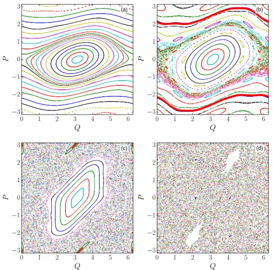
Figure 2.3: Classical phase space for the standard map (2.15) with (a) ε = 0.5, (b) ε = 0.9, (c) ε = 2 and (d) ε = 5.

where we take the perturbation strength as ε = kτ

. This map (2.15) is known as the standard map [Chirikov 1969; 1979], which is regarded as a generic model to exhibit all typical features of Hamiltonian systems.

Figure 2.3 shows the phase space portrait for the standard map. For a weak perturbation regime (ε = 0.5),

most of trajectories follow the regular motions and the phase space is filled with the KAM curves (see

Fig. 2.3(a)). On the other hand, chaotic regions gradually grows with increase in the perturbation strength

ε, and for some intermediate value, say ε = 0.9, the phase space shows very complicated structures with

regular and chaotic orbits (see Fig. 2.3(b)). As discussed in the previous section 2.1, the phase space of

generic Hamiltonian systems typically forms a mixture of regular and chaotic orbits. Such phase space is

called as mixed-type phase space. For a more large ε regime, chaotic regions gradually dominates the phase space, and finally regular regions disappear (see Fig. 2.3(c) and (d)).

For KAM curves in a weak perturbation regime ε, it is possible to introduce a conjugating function which transforms the original dynamics into a constant rotation with rotation numbers ν = Ω/2π, where Ω is the frequency of the classical motion on KAM curves. The conjugating function can be expanded into the Fourier series of the angle variable

q = q(θ) = ∑

k

Q

e

, p = p(θ) = ∑

k

P

e

, (2.16)

which is absolutely convergent for θ ∈ R , according to the KAM theorem. Since a single forward time evolution on the KAM curve leads to a constant shift θ → θ + 2πν, the mapping relation (2.13) requires the following functional equations to hold:

p(θ + 2πν) − p(θ) = − τ d

dq V (q(θ)), q(θ + 2πν) − q(θ) = τ d

dp T (p(θ + 2πν)), (2.17) which can be solved by transforming them into a set of simultaneous algebraic equations for the Fourier coefficients in some cases [Shiromoto et al.]. Especially in the standard map, these coefficients of the Fourier series Q

and P

are expressed using by the double recurrence relation [Greene and Percival 1981]. The solid red curves in Fig. 2.3(b) depict the KAM curve with the golden mean rotation number ν = ( √

5−1)/2, for which the convergence in terms of the continued fractional expansion is the slowest. The KAM tours with the golden mean frequency is believed to be most robust against perturbation and it is known that it breaks at the critical ε = 0.971635 · · · [Greene 1979, Greene and Percival 1981, MacKay 1983]. Invariant tori are break up into so-call cantori [Aubry 1978, Mackay et al. 1984, Percival 1980].

2.3 Quantum dynamics of kicked Hamiltonian

In this section, we consider the quantum dynamics on the surface of section. As is the case in the previous section 2.2, we introduce the quantized kicked Hamiltonian [Casati et al. 1979]

H(ˆ ˆ q, p, t) = ˆ ˆ T (ˆ p) + ˆ V (ˆ q) ∑

n∈Z

τ δ(t − nτ ), (2.18)

where q ˆ and p ˆ are the position and the momentum operators, which satisfy the commutation relation [ˆ q, p] = ˆ i ~ . For the kicked Hamiltonian, the time-dependent Schr¨odinger equation

i ~ ∂

∂t ψ(t) = ˆ H | ψ(t) i , (2.19)

can be integrated from n-th kick to n + 1-th kick over period τ , and the time evolution of wave function

| ψ

i is expressed using the evolution operator U ˆ as

| ψ

i = ˆ U | ψ

i , U ˆ = exp (

− i

~ τ T(ˆ ˆ p) )

exp (

− i

~ τ V ˆ (ˆ q) )

. (2.20)

Since the time evolution (2.20) is also expressed as U ˆ : | ψ

i 7→ | ψ

i , it is often referred to as the quantum maps [Berry et al. 1979, Tabor].

The τ time step evolution starting from an initial condition h q

| ψ

i is given by h q

| ψ

i =

∫

dq

K(q

, q

; τ ) h q

| ψ

i , (2.21) where

K(q

, q

; τ ) ≡ h q

| U ˆ | q

i . (2.22) is the so-called Feynman kernel. By inserting the completeness conditions

∫

dq | q ih q | = 1l, or ∑

q

| q ih q | = 1l, (2.23)

into the Eq. (2.22), the 1 step Feynman kernel can be expressed as h q

| U ˆ | q

i =

∫

dp

h q

| e

| p

ih p

| e

| q

i

= 1 2π ~

∫

dp

exp [ iτ

~

{ q

− q

τ p

− T (p

) − V (q

) }]

= 1 2π ~

∫

dp

exp [ i

~ S

(p

, q

; q

) ]

, (2.24)

where S

stands for the discrete action. The discrete action is expressed as S

= Lτ using a discrete

Lagrangian [Haake, Reichl, Tabor]

L(p

, q

; q

) = q

− q

τ p

− T (p

) − V (q

). (2.25)

We notice that in the continuous time limit τ → 0, the discrete Lagrangian L takes a typical form as

L = p q ˙ − H, (2.26)

via Legendre transformation of the Hamiltonian.

For the multiple time evolution, the Feynman kernel K

(q

, q

) is expressed as K

(q

, q

) ≡ h q

| U ˆ

| q

i

= h q

|

n

∏

[

e

e

] | q

i

=

∫

dq

· · · dq

∫

dp

· · · p

∏

hq

|e

|p

ihp

|e

|q

i

= ( 1

2π ~

)

∫

∏

dq

∫

∏

dp

exp



 iτ

~

n−1

∑

j=0

{ q

− q

τ p

− T (p

) − V (q

) } 

= ( 1

2π ~

)

∫

∏

dq

∫

∏

dp

exp [ i

~ S

( { q

} , { p

} ) ]

(2.27)

where { q

} , { p

} denotes the set of the variable { q

, q

· · · } and { p

, q

· · · } , respectively. Equation (2.27) is nothing less than the Path integral formulation [Feynman and Hibbs, Schulman] for the mapping systems.

Since the dynamics of the quantum map is described as the sequence of the periodic time evolution, the Floquet theorem [Reichl, Saito] allows us to introduce the stationary state under the operator U ˆ , i.e., the eigenvalue u

and eigenstate | Ψ

i are given as

U ˆ | Ψ

i = u

| Ψ

i , (2.28)

where the eigenvalue is expressed as u

= e

and E

is called the quasi-energy. Knowing the

eigenvalues and eigenstates, the Feynman kernel takes another form as K

(q

, q

; τ ) = ∑

m

e

hq

|Ψ

ihΨ

|q

i. (2.29)

Here we use the completeness condition for the eigenstate ∑

m

|Ψ

ihΨ

| = 1l.

As a concrete example, let us consider the eigenvalue problem for the quantized standard map U ˆ , which is given by function T ˆ (ˆ p) = ˆ p

/2 and V ˆ (ˆ q) = k cos ˆ q. Here we impose a periodic boundary condition on the region (q, p) ∈ (0, 2π] × (−π, π]. As a result, the area of the phase space W = 4π

is quantized in units of the effective Planck’s constant

h = W/N, (2.30)

where N is the dimension of the Hilbert space of the system.

In order to visualize wave function in the phase space, we introduce the Husimi-representation which is given by the projection of the wave function onto the coherent state

h q | α(q

, p

) i = ( 1

π ~

)

e

, (2.31) whose center is (q

, p

). The Husimi-representation is given by

ρ

(q, p) = |h α(q, p) | Ψ i|

, (2.32)

and it represents a quasi-probability density in the phase space.

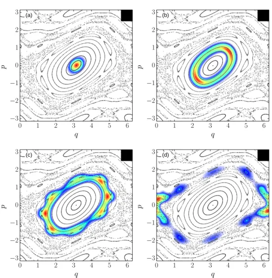
Figure 2.4 shows the eigenstate |Ψ

i in the Husimi-representation. As shown in Figs. 2.4(a) and (b), some eigenstates have their supports on the corresponding elliptic invariant curves. As can be seen in Fig. 2.4(c) and (d), on the other hand, the support of some other eigenstates |Ψ

i are not invariant curves but classical resonances, specified such as 1 : 8, in case (c), and the chaotic region in case (d).

For the systems with mixed phase space, the semiclassical eigenfunction hypothesis [Berry 1977, Per-

cival 1973] implies that each eigenstate |Ψ

i has a support either on a regular or on a chaotic region in

the semiclassical limit ~ → 0. For the finite ~ regime, on the other hand, the wave function spreads over

the classical invariant curves and so the transition between regular and chaotic regions is not forbidden.

0 1 2 3 4 5 6

q

− 3

− 2

− 1 0 1 2 3

p

(a)

0 1 2 3 4 5 6

q

− 3

− 2

− 1 0 1 2 3

p

(b)

0 1 2 3 4 5 6

q

− 3

− 2

− 1 0 1 2 3

p

(c)

0 1 2 3 4 5 6

q

− 3

− 2

− 1 0 1 2 3

p

(d)

Figure 2.4: Some eigenstates in the Husimi-representation for quantized standard map with k = 1. Upper

right box represents the size of effective Planck’s cell h.

Such a process is dynamical tunneling [Davis and Heller 1981, Keshavamurthy and Schlagheck 2011] as a

generalization of the potential barrier tunneling.

Theory of tunneling splitting

The tunneling effect is peculiar to quantum mechanics and no counterparts exist in classical mechanics. The most important qualitative difference between one-and multi-dimensional sys- tems would be that classical particles are confined not only by the energy barrier, but also by the dynamical barrier as discussed in the previous chapter 2. What is more crucial is the fact that generic multi-dimensional systems are no more completely integrable and chaos appears in the underlying classical dynamics, so one must take into account new aspects of quantum tunneling absent in completely integrable systems [Creagh 1998, Keshavamurthy and Schlagheck 2011].

In this chapter, we will consider the tunneling effect of the eigenstates. Before consideration is given to non-integrable systems, we will explain the tunneling splitting in section 3.1, which will be use to measure quantum tunneling quantitatively. In section 3.2, we will briefly review the theory resonance-assisted tunneling [Brodier et al. 2002, Schlagheck et al. 2011], which especially attracts a great deal of attention since it explains various important features of tun- neling in non-integrable systems. In section 3.3, we outline the semiclassical description for resonance-assisted tunneling in integrable system [Le Deunff et al. 2013]. Then we will discuss the validity of applying resonance-assisted tunneling scenario to non-integrable systems.

19

−2 −1 0 1 2 q

0.0 0.2 0.4 0.6 0.8 1.0 1.2 1.4

V ( q ) , |h q | Ψ

i|

(a)

−2 −1 0 1 2

q 10

10

10

10

10

10

10

10

10

10

|h q | Ψ

i|

(b)

n= 0 n= 4 n= 10

-1 0 1 ^q

-1 0 1

p

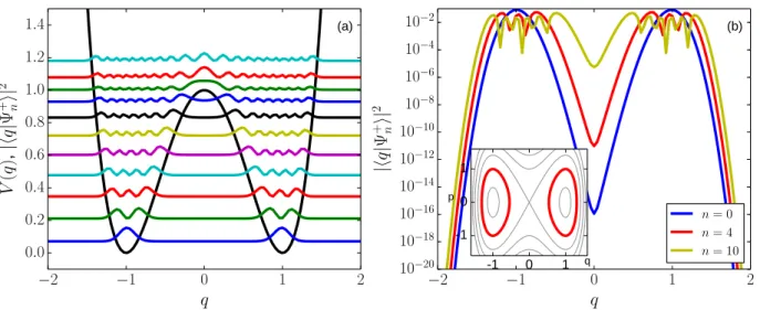
Figure 3.1: The eigenstate | Ψ

i in the q-representation for the double well potential with a = 1 in (a) normal scale and (b) semi-log scale. The inset of (b) shows the classical phase space and the red curve draws energy contour with E = 1/2.

3.1 Tunneling splitting in the double well system

In this section, we will consider quantum tunneling observed in the eigenstates. For tunneling in eigen- states, the energy splitting associated with the symmetry of the potential function is often discussed. We explain some basic aspects of the tunneling splitting using a one-dimensional double well system, for which Hamiltonian is expressed as

H(q, p) = p

2 + V (q), (3.1)

with the potential function

V (q) = (q

− a)

. (3.2)

When the energy is less than the local maximum E < a

, classical trajectories in phase space form an elliptic curves which means that the (real) classical dynamics cannot go over the potential barrier (see the red curve in the inset of Fig. 3.1(b)). On the other hand, the wave packet can penetrate the potential barrier, and such a purely quantum effect is usually referred to as tunneling.

We consider the tunneling problem for eigenstates in the double well system. We denote the eigenvalue equation by

H|Ψ ˆ

i = E

|Ψ

i. (3.3)

The potential function (3.2) is symmetric with respect to the q-axis, so the eigenstate is also symmetric with respect to the q-axis, that Ψ

(q) = ± Ψ

( − q) is satisfied. Figure 3.1 demonstrates the eigenstates

| Ψ

i which have numerically been obtained. In the following discussion we consider the approximate construction of the eigenstate | Ψ

i

based on WKB theory, whose procedure follows a standard textbook such as [Landau and Lifshits].

We assume that Ψ

(q) is a local WKB solution only in the right-hand side q ≥ 0 with energy E

. Here the local solution is normalized in the right-hand side as ∫

0

| Ψ

(q) |

= 1. The eigenstates Ψ

(q) of the system are given as a linear combination of the local WKB solution

Ψ

(q) ' 1

√ 2 (Ψ

(q) + Ψ

(−q)) , (3.4) Ψ

(q) ' 1

√ 2 (Ψ

(q) − Ψ

( − q)) . (3.5)

These relations lead that at q = 0

Ψ

(0) = √

2Ψ

(0), Ψ

(0) = 0, (3.6a)

Ψ

(0) = 0, Ψ

(0) = √

2Ψ

(0), (3.6b)

and ∫

0

Ψ

(x)Ψ

dq ≈

∫

0

| Ψ

(q) |

dq = 1/ √

2. (3.6c)

Here the prime stands for the derivative with respect to q. The Schr¨odinger equation for the eigenstates Ψ

(q) and Ψ

(q) is given as

Ψ

(q) + 2

~

(E

− V (q))Ψ

(q) = 0, (3.7a) Ψ

(q) + 2

~

(E

− V (q))Ψ

(q) = 0. (3.7b) By multiplying (3.7a) by Ψ

and (3.7b) by Ψ

and subtracting from each other, we find

2

~

(E

− E

)Ψ

(q)Ψ

(q) = Ψ

(q)Ψ

(q) − Ψ

(q)Ψ

(q). (3.8)

1

In the following discussion, we drop the quantum number n.

2

Ψ

(q) is also a local solution in the left-hand side (q ≤ 0) with energy E

due to the symmetry.

Integrating the both side of Eq. (3.8) from 0 to ∞, we find

√ 2

~

(E

− E

) =

∫

0

Ψ

(q)Ψ

(q) − Ψ

(q)Ψ

(q) dq

= [Ψ

Ψ

− Ψ

Ψ

]

−

∫

0

Ψ

(q)Ψ

(q) − Ψ

(q)Ψ

(q) dq, (3.9) and

E

− E

= −~

Ψ

(0)Ψ

(0), (3.10a) E

− E

= ~

Ψ

(0)Ψ

(0). (3.10b) Therefore the energy of the symmetric and antisymmetric state |Ψ

i slightly shifts from E

and the amount of the energy shift is given by

∆E := E

− E

' 2 ~

Ψ

(0)Ψ

(0), (3.11) where ∆E is referred to as tunneling splitting, which is regarded as representing tunneling probability for the wave packet to penetrate the potential barrier.

The splitting formula (3.11) can also be interpreted via WKB (semiclassical) wave function. The eigen- function and its derivative in the classical forbidden region is expressed semiclassically as

Ψ

(q) =

√ Ω 2πp(q) exp

(

− 1

~

∫

0

|p(q

)| dq

)

, Ψ

(q) = p(q)

~ Ψ

(q), (3.12) where p(q) = ± √

2(E − V (q)) and t

is a turning point [Landau and Lifshits]. Here Ω is the frequency for the oscillation of the particle. Note that the p(q) takes a pure imaginary value between − t

< q < t

. Using Eq. (3.12), the tunneling splitting is semiclassically expressed as

∆E ∼ Ae

, (3.13)

where the amplitude factor A and the classical action S are respectively given as A = Ω~

π , S =

∫

−tp

|p(q

)| dq

. (3.14)

Here the classical action S is referred to as the instanton action [Coleman 1988]. This formula tells us that the tunneling splitting ∆E decays exponentially as a function of 1/ ~ . This is a reasonable result because the tunneling effect is supposed to be exponentially small and vanish in the semiclassical limit ~ → 0. We also notice that using the Eq. (3.12) the tunneling splitting could be written as

∆E ∼ 2 ~ p(0)Ψ

(0) = ~ p(0)Ψ

(0), (3.15) where we have used the relation (3.6) at q = 0. Therefore, the splitting ∆E correlates with the amplitude of the symmetric eigenstate Ψ

(q) at q = 0. The splitting formula in multidimensional (quasi-)integrable systems without classical resonances, has been derived in [Wilkinson 1986] as

∆E ∼ Ae

, (3.16)

where the amplitude factor A is in proportion to ~

and S denotes the instanton action in multi-dimensional space.

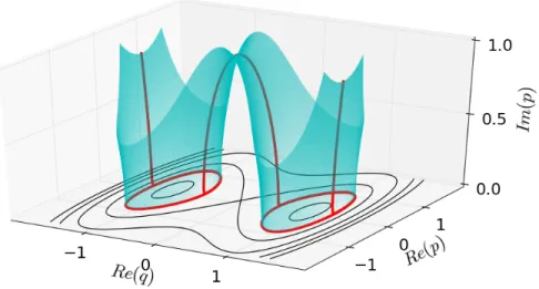
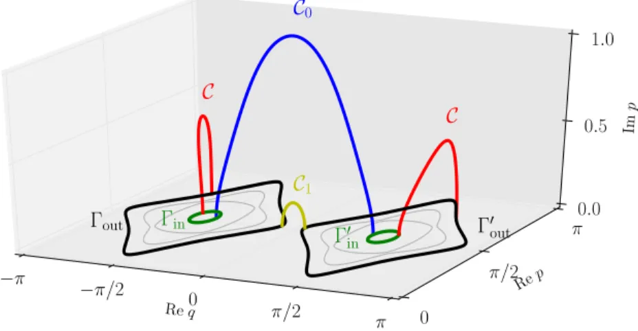
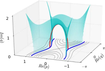
Figure 3.2 shows the analytic continuation of the curve p(q) = ± √

2(E − V (q)), V (q) = (q

− 1)

, (3.17) into the imaginary energy. In Eq. (3.17), the integration between turning points − t

< q < t

is evaluated along the red curve whose imaginary energy is zero. The so-call instanton path is a complex orbit connecting the symmetrically situated two wells.

So far, we have derived the tunneling splitting based on the eigenstate in the q-representation. For the

convenience of the formulation, we here provide another derivation for the tunneling splitting. We assume a

one dimensional time-independent Hamiltonian H that exhibits two main symmetric regions in phase space,

in analogy with the double well system. Suppose the local WKB solution of the left |Li and right |Ri wells

Figure 3.2: The analytic continuation of the curve (3.17) for the real energy E = 1/2. The cyan surface has an imaginary energy and the red curves represent the manifolds with a real energy.

with degenerate energy E

. The eigenstates | Ψ

i of the Hamiltonian H are given as a linear combination

| Ψ

i ' 1

√ 2 ( | L i ± | R i ). (3.18)

This suggests that the Hamiltonian H ˆ is simply expressed by the two-dimensional matrix in which | L i and

| R i are taken as the basis functions has. The corresponding energies E

are given as

h Ψ

| H ˆ | Ψ

i = E

. (3.19)

Substituting |Ψ

i given in (3.18) into Eq. (3.19), E

' 1

2 h L ± R | H ˆ | L ± R i

= 1 2

( hL| H|Li ˆ + hR| H|Ri ± hL| ˆ H|Ri ± hR| ˆ H|Li ˆ )

= 1 2

(

2E

+ h L | H ˆ − H ˆ

| L i + h R | H ˆ − H ˆ

| R i ± 2 h L | H ˆ | R i . )

(3.20)

Subtracting from each other, the energy splitting

∆E = E

− E

' 2hL| H|Ri, ˆ (3.21)

is evaluated as the off-diagonal term. The diagonal matrix elements are given as h L | H ˆ | L i ' 1

2 h Ψ

+ Ψ

| H ˆ | Ψ

+ Ψ

i

= 1 2

( h Ψ

| H ˆ | Ψ

i + h Ψ

| H ˆ | Ψ

i + 2 h Ψ

| H ˆ | Ψ

i )

= 1 2

( E

+ E

)

= E

' hR| H|Ri. ˆ (3.22)

Therefore the Hamiltonian matrix is represented by

H ˆ =



 E

∆E/2

∆E/2 E



 , (3.23)

and the eigenvalues are expressed as E

± ∆E/2 as expected.

Now we consider the dynamics of the state | R i , which localizes in the right-hand side of the well. The time-evolution of | R i is expressed as

|ψ(t)i = e

|Ri = 1

√ 2 (

e

|Ψ

i + e

|Ψ

i )

= 1 2 e

{

e

( | R i + | L i ) + e

( | R i − | L i ) }

= e

{

cos ( ∆E

2~ t )

| R i + i sin ( ∆E

2~ t )

| L i }

. (3.24)

At t = π ~ /∆E, the right state | R i moves to the left state | L i. Therefore the state | R i periodically oscillates between the two wells with period of

T = h

∆E . (3.25)

−6 −4 −2 0 2 4 6

q

−3

−2

−1 0 1 2 3

p

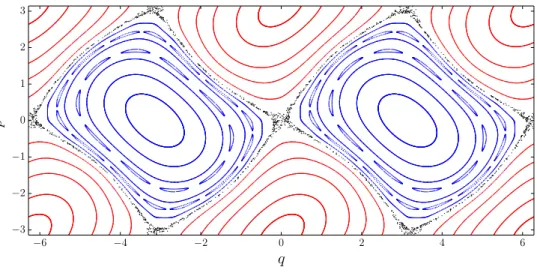
Figure 3.3: The classical phase space of the Harper map corresponding to Eq. (3.26)

3.2 Resonance-assisted tunneling

A two level approach in Eq. (3.23) breaks down, if the chaotic region appears in the phase space. The role of chaos in quantum tunneling has first been discussed in the observation of the wave packet dynamics [Lin and Ballentine 1990], and then is clearly recognized in the behavior of the tunneling splitting of eigenenergies [Bohigas et al. 1990; 1993a;b, Roncaglia et al. 1994, Tomsovic and Ullmo 1994]. In non-integrable systems, a doublet forming a tunneling splitting is not isolated in the whole energy space. It can happen that the states forming a doublet and a state supported by the chaotic region come close to each other and form avoided crossings. Within the interaction regime of energy resonance, the energy splitting between the doublet becomes large through the coupling with the chaotic state, meaning that the tunneling amplitude between one tours to the other is enhanced. Chaos-assisted tunneling (CAT) occurs in this way [Bohigas et al.

1993b, Tomsovic and Ullmo 1994]. The enhancement of the tunneling due to the energy level resonance is often called resonant tunneling, which is reduced to a one-dimensional triple-well potential [Le Deunff and Mouchet 2010, Schlagheck et al. 2011].

A more direct explanation for the tunneling in non-integrable systems was given based on the time- domain semiclassical analysis [Onishi et al. 2003, Shudo and Ikeda 1994; 1995; 1998, Shudo et al. 2009a;b].

In particular, the complex dynamical systems could explain the tunneling effect in non-integrable systems.

This semiclassical analysis tells us that exponentially many complex orbits connecting the tours and chaotic

region give rise to the enhancement of the tunneling probability. This tunneling effect is called chaotic tunneling. Especially, chaos in complex domain, the so-called Julia sets, plays a fundamental role in the tunneling in non-integrable systems [Shudo et al. 2009a;b].

The enhancement of the tunneling probability has been reported not only in the strongly chaotic regime but also in the nearly-integrable regime. The phase space of the latter is almost filled with KAM tori like Fig. 3.3. Such enhancement of the tunneling splitting was first reported by [Roncaglia et al. 1994]. Then the authors of Ref. [Bonci et al. 1998] pointed out that the energy level resonances are induced by not only chaos but classical nonlinear resonances.

The authors of Ref. [Brodier et al. 2001; 2002] conjectured that the complexified KAM curve does not seem to provide an appropriate frame work for the semiclassical study of nearly-integrable regime, because the analytic continuations of the invariant KAM curve with each symmetric wells do not meet each other unlike the double well potential system (see Fig. 3.2). In general, KAM curves specified as Eq. (2.16) has the radius of convergence in complex angle variable at θ

and singularities accumulate along θ

[Berretti and Chierchia 1990, Berretti et al. 1992, Greene and Percival 1981]. Such a border of analyticity is conjectured to form the natural boundary. The instanton connection along the complexified KAM curve is interrupted by the natural boundary of the KAM curve. (This topic revisits in section 4.1)

Instead of overcoming issues arising from the existence of the natural boundary, the authors of Ref. [Brodier et al. 2002] investigated the coupling mechanism between low lying and excited states, which is referred to as resonance-assisted tunneling (RAT). RAT has been shown to successfully reproduce the splitting curve not only in the nearly-integrable regime but also in the strongly chaotic regime [Eltschka and Schlagheck 2005, Keshavamurthy 2005, L¨ock et al. 2010, Mouchet et al. 2006, Schlagheck et al. 2011, Sheinman et al.

2006]. We should note that the study of tunneling in the system with nonlinear resonances was first made in the work of [Ozorio de Almeida 1984]. So far, it has been believed that the origin of the enhancement of the splitting could be explained in the framework of RAT.

Before we explain theory of RAT more precisely, we actually demonstrate how the enhancement of tunneling splitting is observed in non-integrable systems. Let us consider the quantized Harper map

U ˆ = exp ( i

~ cos ˆ p )

exp ( i

~ cos ˆ q )

, (3.26)

0.0 0.5 1.0 1.5 2.0 2.5

1/h

10⁻⁴⁰ 10⁻³⁷ 10⁻³⁴ 10⁻³¹ 10⁻²⁸ 10⁻²⁵ 10⁻²² 10⁻¹⁹ 10⁻¹⁶ 10⁻¹³ 10⁻¹⁰ 10⁻⁷ 10⁻⁴ 10⁻¹

| ∆ E

|

(A) (B)

(C) (D)

integrable τ= 1

−7

−6

−5

−4

−3

−2

−1 0

|hq|Ψ0i|2,(log10)

integrable (A) −10

−8

−6

−4

−2 0

integrable (B)

−3 −2−1 0 1 2 3

q

−16

−14

−12

−10

−8

−6

−4

−2 0

|hq|Ψ0i|2,(log10)

integrable (C)

−3−2 −1 0 1 2 3

q

−20

−15

−10

−5 0

integrable (D)

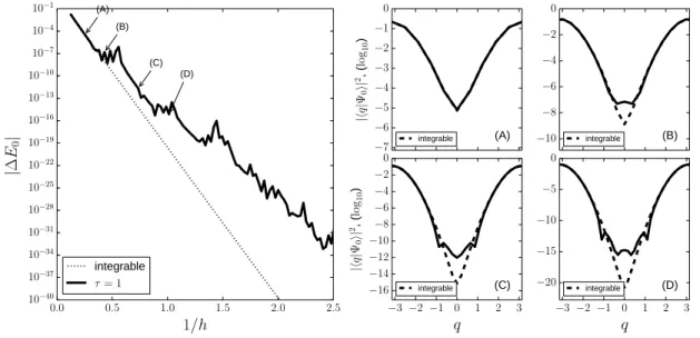
Figure 3.4: Left panel shows the tunneling splitting ∆E

as a function of the effective Planck’s constant 1/h for the ground state and first excited of the quantized Harper map with τ = 1. Dashed curve denotes the tunneling splitting for the associated integrable Hamiltonian H ˆ

with M = 5. Right panels (A)-(D) show the eigenstate | Ψ

i in q-representation with 1/h, each of which is indicated in the Left panel.

for which the associated classical phase space is shown in Fig. 3.3. We then consider the tunnel splitting

∆E of bounded states localizing at (q, p) = ( ± π, 0). Left panel in Fig. 3.4 shows the tunneling splitting as a function of the effective Planck’s constant 1/h. For reference, Fig. 3.4 shows the splitting of the cor- responding integrable one, which is given by the effective integrable Hamiltonian H ˆ

(see Appendix B).

We notice that the tunneling splitting ∆E in a small 1/h regime for the quantized Harper map coincides with that of the integrable one. On the other hand, the splitting ∆E in the Harper map becomes larger than that in the corresponding integrable one by several orders of magnitude. The splitting curve typically forms plateaus accompanied by spikes due to the energy resonance and rapidly decaying region. We refer to the structure of plateau and rapidly decaying region as the staircase structure. It would be worth mentioning that the characteristic pattern of the eigenstate appears around q = 0: the eigenstate takes a convex structure in the plateau of the splitting curve (see Fig. 3.4(B) and (D))

, and a concave structure in the rapidly decaying regime (see Fig. 3.4(A) and (C)).

In what follows, we review RAT theory developed in [Brodier et al. 2002, Schlagheck et al. 2011]. As

3

In Fig. 3.4(A), the convex structure is difficult to see but it possible to decompose the component which makes a convex

structure using contribution decomposition discussed in sections 4.2 and 5.3