Generalization of Central Place Theory Using Mathematical Programming

(1)

Generalization of Central Place Theory Using Mathematical Programming

Kenji ISHIZAKI

2015

(2)

i

3.2 Combinational problem of the superimposition of market area networks 39 3.3 The superimposition problem as a combinatorial optimization 43 3.4 Comparing the Lösch’s system with the solution of model 46 3.5 Testing the rationality of constructing a hierarchy on Lösch’s system 49 3.6 Hierarchical arrangement based on the agglomeration effect 52

3.7 Testing the agglomeration effect 57

4 Generalization of central place theory

⁶³

(3)

ii

4.1 Reinterpreting central place theory from the perspective of the locational

principle 63

4.2 Christaller’s central place theory as a superimposition problem for market area

networks 71

4.3 Generalized model of central place theory 77

5 Conclusion

⁸¹

References

⁸⁷

(4)

iii

List of Figures

Figure 1 Concept of demand cone 6

Figure 2 Löschian locational equilibrium in a linear market 7 Figure 3 Potential solutions of the locational competition by three firms in a

bounded market 9

Figure 4 Hypothetical linear market and uniform and non-uniform distributions of

population 17

Figure 5 Demand allocation pattern near the boundary 19

Figure 6 Solutions of the total demand maximization problem in a linear market 22 Figure 7 Solutions of the total demand maximization problem in a plane market 25 Figure 8 Solutions of the total profit maximization problem in a linear market 29 Figure 9 Locational pattern of non-inferior Solution C in Table 1 32

Figure 10 Derivation of the market areas of various sizes 36

Figure 11 Superimposition of market area networks of the Lösch’s system 38 Figure 12 Market area network obtained by moving the market center to another

point from a metropolis 41

Figure 13 Central place systems of one hundred fifty market area networks 47 Figure 14 Distribution of market centers for market area Number 6 50 Figure 15 Solutions of the model based on the agglomeration effect 58

Figure 16 Agglomeration by the neighborhood effect 59

Figure 17 Superimposition of market area networks of the Christaller’s system 72 Figure 18 Non-inferior solutions of the generalized model using multiobjective

programming 75

(5)

iv

List of Tables

Table 1 Non-inferior solutions of the extended model for single good 32

Table 2 List of fifty-five market area networks 39

Table 3 Comparison of the sectors in the Lösch’s system and the solution of model 48 Table 4 Relationship between types and effects of agglomeration in the case of

four kinds of goods 54

Table 5 Classification of the extended model based on locational principles 66

(6)

v

Abstract

Central place theory that is the theory of location of urban settlements where goods and services are supplied was established by Walter Christaller in 1933, and expanded by August Lösch seven years later. The purpose of this thesis is to reinterpret their theories that have been forced to rely on descriptive and geometrical explanations from mathematical modelling perspective. Specifically, modelling for both of the locational principle of single good and the superimposition problem of market area networks are attempted by using mathematical programming comprising some constraints and an objective function. Moreover, the generalized model that both of the locational principle and the hierarchical structure are integrated is presented, and Lösch's and Christaller's theories are identified systematically on the generalized model.

First of all, the market area theory of Lösch as a location problem of single good was modeled, and the extended model was developed in Chapter 2. When the process of locational equilibrium of firms based on the concept of demand cone and the normal profit is premised, the market area theory of Lösch can be formulated as the total demand maximization problem. In the previous studies concerning modelling the theory of Lösch, there were some problems in the formulation to reproduce theoretical central place system for the conditions such as assuming the behavior of firm and deriving the appropriate market area. On the other hand, the model of this thesis is able to reproduce the original Lösch’s theory because of formulating an objective to maximize total demand subject to the conditions of the nearest center hypothesis and the indifference principle. According to the results of applying the model in hypothetical areas, the model will be considered as an operational model of the market area theory of Lösch that enables the derivation of a realistic central place system under the more relaxed assumptions such as non-uniform

(7)

vi

population distribution. However, the firm obtains only the normal profit in the market area theory of Lösch that requires the free entry and the perfect competition to the market. Then, the total profit maximization problem that is antithetic to the total demand maximization problem was examined in consideration of realistic firm's behavior, and the two objectives were integrated by using multiobjective programming as the extension of the model for single good. The extended model is able to be regarded as a flexible model in handling the number of firms concerning the locational principle according to the results of applying in a hypothetical area.

Next, the method of constructing a hierarchy in Lösch’s market area theory was examined, and the mathematical formulation of the superimposition problem of market area networks was attempted in Chapter 3. On the basis of the interpretation in the previous studies concerning the hierarchical arrangement of Lösch, it has been considered that two conditions of prioritizing location in particular sectors and maximizing the number of coincident market centers are the objectives of constructing a hierarchy. Then, the model that optimizes these two objectives was formulated as a combinatorial optimization and applied to the discrete lattice network of regular equilateral triangles. As a result, the central place system by Lösch was not reproduced, and the solution of the model was optimal for the purpose of prioritization of locating in particular sectors. Namely, it has been understood that the perspective towards the rationality of the entire system was lack from Lösch's process of constructing a hierarchy. Then, this thesis attempted to reinterpret Lösch's original intention in constructing a hierarchy, and developed the extended model based on the agglomeration effects. The application of the extended model revealed that the priority location in a particular sector was not an essential condition of the agglomeration of goods and the agglomeration effect by setting neighborhood ranges was able to derive more realistic central place hierarchy.

(8)

vii

In Chapter 4, Christaller’s central place theory was reinterpreted based on the extended models both of the locational principle of single good and the hierarchical arrangement in the market area theory by Lösch. It is the core of a subject in this thesis to identify Christaller's and Lösch's theories systematically according to the extended models. When the objective function in the extended model of single good was expanded, the problem divided into three objectives—the maximum coverage of demand, the minimization of total distance traveled, and the minimization of the number of locations. From the perspective of the locational principle by combining three objectives, Christaller's central place theory was able to be identified as a generalized median problem in which second and third objectives are integrated. Because the generalized median problem is formulated as multiobjective programming, a different number of firms can be assumed in the case of one kind of good supply. Therefore, Christaller's central place theory was identified as the superimposition problem that one kind of good was associated with multiple market area networks. The application of the extended model for hierarchical arrangement indicated that central place system based on Christaller’s marketing principle was reproduced when the agglomeration effect was prioritized.

Consequently, in this thesis, the generalized model of central place theory was presented by integrating the models both of the locational principle of single good and the hierarchical arrangement. When Lösch’s and Christaller's theories are identified using the generalized model, we can recognize that the former precedes the locational principle for single good while the latter prioritizes the agglomeration effect of goods. However, central place systems based on various locational principles and flexible hierarchical structures will be assumed in the real world. The generalized model of central place theory presented in this thesis is able to be considered as an analytical model that would be the touchstone of original theories to the real-world central place system.

(9)

viii

(10)

ix

Acknowledgements

I would like to express my special appreciation and thanks to Professor Yoshio Sugiura for his encouragement of my research. If I had not encountered him in my undergraduate days of Tokyo Metropolitan University, I would not have pursued a career as a researcher. I am grateful for his allowing me to grow as a geographer and for his supporting generously for a long time. I would also like to thank Professor Yoshiki Wakabayashi and Associate Professor Akihiro Takinami for their incisive and helpful comments. I have been indebted to my current colleagues at Nara Women’s University and my former colleagues at Tokyo Metropolitan University. Lastly, I dedicate this thesis to my family and my parents.

Although my father passed away in June 2010 before the completion of this thesis, he was the one who wished for receiving my doctoral degree. I am sure that he is keeping an eye on me from heaven.

(11)

1

CHAPTER 1 Introduction

Central place theory—a theory for explaining the number, size and distribution of urban settlements that provide goods and services to its surrounding area—was initially established in 1933 by Walter Christaller in Die zentralen Orte in Süddeutschland, and later expanded in 1940 as a general schema of central place systems in the market area theory developed by August Lösch. In the history of human geography, central place theory is one of the classical location theories, and has been the subject of research that many geographers attempted to apply with quantitative analysis after the Quantitative Revolution. For instance, there are many literatures such as the empirical studies on the hierarchical structure of central place systems using multivariate statistical analysis (e.g., Berry and Barnum 1962; Beavon 1972), the theoretical studies on the geometric characteristics of systems (e.g., Dacey 1965; Arlinghaus 1985), and the mathematical approaches to dynamic model of central places (e.g., Allen and Sanglier 1981; Clarke and Wilson 1985). Of mathematical techniques, location-allocation models for solving the facility location problem ‘provide a suitable tool for operationalizing the concepts of central place theory’ (Beaumont 1987: 21) because of generating alternate spatial structure of central place systems by varying different assumptions (Ghosh and Rushton 1987).

Location-allocation model is stated using mathematical programming formulation to seek the optimal location subject to constraints such as consumer and producer behaviors. Mathematical programming formulation is an effective method for modelling central place theory that founded on optimality principle (Beaumont 1982). Attempts to model central place theory using mathematical programming include studies, such as those of Henderson (1972), Dökmeci (1973), Puryear (1975), and Kohsaka (1983), that have sought to develop analytical models by taking advantage of the

(12)

2

frameworks of central place theory, as well as those that have sought to reproduce theoretical central place systems, such as those of Storbeck (1988, 1990), Kuby (1989), and Curtin and Church (2007).

While these studies have incorporated mathematical programming as a means of deriving the hierarchical spatial arrangement of central places, their examination of the assumptions and locational principles of central place theory is inadequate, and they cannot necessarily be said to have faithfully replicated the original central place theory (Ishizaki 1992). If we are to consider the role of central place theory as an operational model, then we need to first of all examine the nature of the constraints and objectives that Christaller and Lösch imposed on their theory when deriving their central place systems (Beaumont 1982: 239).

However, both Christaller’s and Lösch’s discussion, despite their relatively rigorous discussion before deriving the schema of central place system, such as for example in their discussion of supply and demand relationship of goods and services, becomes vague when actually locating central places or firms and consequently constructing the hierarchical structure. This ambiguity has often led to misinterpretations of the theory (e.g., Berry and Garrison 1958a) and has resulted in the faithful understandings of the original theory (Saey 1973; Beavon 1977; Morikawa 1980; Hayashi 1986). It is necessary to read between the lines in the writings of Christaller and Lösch in order to supplement the inherent ambiguity and insufficient explanation in the original central place theory. Whereas their theories have previously been forced to rely on descriptive and geometric explanations, today, in an era marked by significant advances in the elaboration of mathematical models and computerized numerical analysis, I am confident that their reconceptualization from a mathematical modeling perspective can provide new insights into central place theory.

The purpose of this paper is to develop a model that reproduces central place systems using mathematical programming and to reinterpret Christaller’s and Lösch’s theories through the process of constructing the generalized models. Especially, this paper focuses on modeling of Lösch’s theory because Ishizaki (1995) has previously attempted to develop the model of Christaller’s central place

(13)

3

theory. Furthermore, after the model of Lösch’s theory is extended, the differences between Christaller’s and Lösch’s theories are examined according to an extended model.

Chapter 2 attempts to model Lösch’s market area theory in the location of single good, and then, on the basis of the results of applying the model in a hypothetical area, it is examined whether the Lösch’s system can be reproduced according to the operational model of the theory. Although Kuby (1989) has already attempted to model Lösch’s market area theory, there appears to be a number of problems with its formulation in Kuby (1989) concerning the model’s validity. Hence, after critically examining Kuby’s model, the model of Lösch’s theory is reformulated on the basis of reinterpretation of the theory. Thereafter, after establishing an objective antithetical to Lösch’s theory, an extension of the model concerning the location of single good is developed by unifying the two objectives.

Chapter 3 discusses the method of constructing a hierarchy in Lösch’s market area theory and attempts to model the superimposition problems of hexagonal networks. The hierarchical properties of Lösch’s system were intensely debated by Beavon, Marshall, and others in the 1970s (cf. Tarrant 1973; Beavon and Mabin 1975; Haites 1976; Marshall 1977, 1978a, 1978b; Beavon 1978a, 1978b), which resulted in the clarification of a number of things, including a method for faithfully reproducing Lösch’s central place systems and the geometrical and mathematical characteristics of hexagonal networks. However, there is a problem that has been overlooked in the discussions of these scholars.

Namely, this problem is concerned with the rationality of Lösch’s central place system from the perspective of optimal hierarchical structure. That is, there is no single method for constructing a hierarchy by superimposing multiple hexagonal networks of market areas because of the enormous possible combinations of central place systems. This rationality of the scheme presented by Lösch can be verified by comparing with the solutions of model. Furthermore, this chapter presents the reinterpretation concerning the objective of constructing a hierarchy in Lösch’s theory and attempts to extend the model considering the agglomeration effect of hierarchical central place systems.

In Chapter 4, based on the extended model related to the location of single good obtained in

(14)

4

Chapter 2 and the extended model of hierarchical structure obtained in Chapter 3, the differences between Lösch’s and Christaller’s theories are clarified and both theories are generalized by the unified model. Whereas Lösch’s theory is required to make a hexagonal market area network, whose size is unique to each good, correspond to that good on the basis of the concept of thresholds, Christaller’s central place systems are based on the concept of the range of goods and the successively inclusive hierarchy (Schultz 1970), and while both have the same hexagonal structure, the latter differs from the former in terms of the locational principle and hierarchical structure. Therefore, this chapter attempts to reinterpret the locational principle in Lösch’s and Christaller’s theories on the basis of an extended model related to the location of single good, and reveals that it is possible to derive Christaller’s central place systems using the extended model of hierarchical structure. On the basis of these findings, a generalized model that integrates the location problems of single good and the hierarchical structure is proposed using multiobjective programming. I am convinced that there is yet no attempt to integrate of both central place theories as viewed from the model structure using multiobjective programming.

(15)

5

CHAPTER 2 Modelling and extending Lösch’s theory in the location problems of single good

2.1 The concept of demand cone and the location of firm

According to Lösch, the equilibrium of locations “is determined by two fundamental tendencies:

the tendency as seen from the standpoint of the individual firm and hitherto alone considered, to the maximization of advantages; and, as seen from the standpoint of the economy as a whole, the tendency to maximization of the number of independent economic units” (Lösch 1954: 94). In other words, as a result of the free entry of a large number of firms in pursuit of profit, the entry of firms ends at the point where normal profit is mutually obtained, creating a state of locational equilibrium.

At this point, the number of firms that have entered the market is maximized.

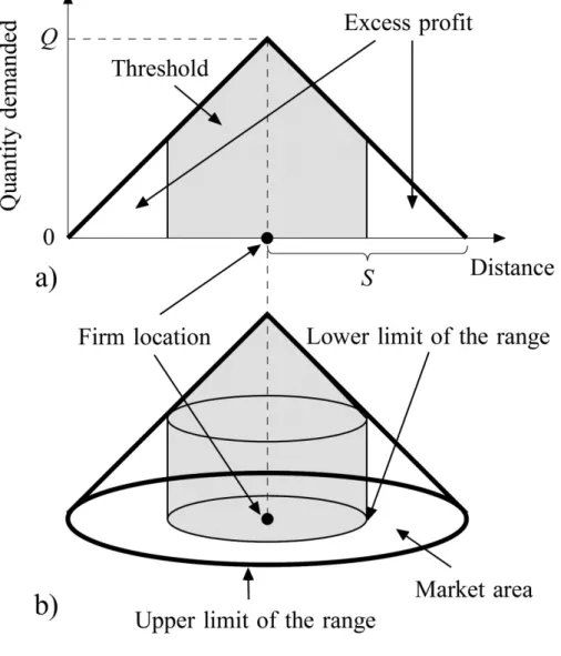
The concept of market area, which is based on demand cones, has been introduced to consider the process of locational equilibrium as a spatial perspective. Figure 1 shows a schematic representation of demand cones for linear market (Figure 1-a) and two-dimensional market (Figure 1-b). In Figure 1, Q represents maximum demand, with demand falling in proportion to the distance of a particular good from the firm location, such that demand falls to zero at distance S, which represents the upper limit of the range of a good. When a firm is able to monopolize a two-dimensional market, the market area of the firm in that market transforms to a circle with a radius S. However, assuming the case where a large number of competitors have entered the market, there is a possibility that firms will be unable to secure a circular market area with radius S. This is because, in the case that a profit can be obtained from a market area even if it overlaps with that of a competitor, a new firm can enter in close proximity, resulting in the reduction of the market area.

The minimum demand necessary in order for firms to remain in business is known as “threshold”

(16)

6

(Berry and Garrison 1958b), and where there is a uniform distribution of population and households, the threshold can be expressed as the area or volume of the shaded part of Figure 1. Therefore, if a firm’s threshold falls below the total demand (i.e., the whole area or whole volume of the demand cone in Figure 1), then other firms will be able to establish locations up to the point where a firm is able to secure the threshold.

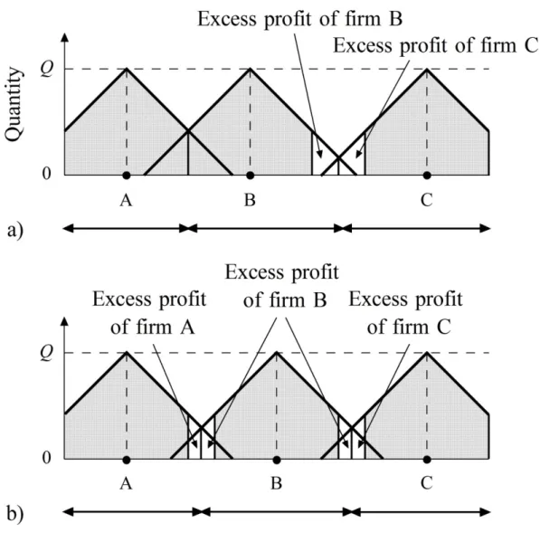
Figure 2 represents linear market situations in which each firm is able to obtain maximum excess profit (Figure 2-a) or only normal profit (Figure 2-b), with the market area for each firm shrinking in

Figure 1 Concept of demand cone

(17)

7

the process of shifting from the situation in Figure 2-a to the situation in Figure 2-b. Here, the situation in Figure 2-b represents the solution to the locational equilibrium process by Lösch. Assuming an infinitely spreading linear market with a uniform population distribution, firms appear at equal intervals securing market areas in which they can obtain a normal profit, which achieves the maximum number of firms in the market.

The case of a two-dimensional market is rather more complicated in that market areas overlap Figure 2 Löschian locational equilibrium in a linear market

The right side of a linear market is assumed to extend infinitely.

(18)

8

with one another between the locations of surrounding firms, and because the base of the demand cone is cut off, the shape of the market area is polygonal rather than circular. Of all polygons able to fill a plane, the regular hexagon is able to obtain the most efficient demand (Lösch 1954: 111), therefore, when the distribution of population is uniform, a honeycomb-like market area network comprising regular hexagons of identical size that satisfies the threshold is formed.

2.2 Problems with Kuby’s formulation

Kuby (1989) attempts to model Lösch’s locational equilibrium process by defining the objective of maximizing the number of firms while satisfying threshold constraints as an optimization problem.

This formulation is regarded as a model that reproduces Lösch’s system relatively precisely. However, there are several problems with Kuby’s formulation as an operational model of the original central place theory.

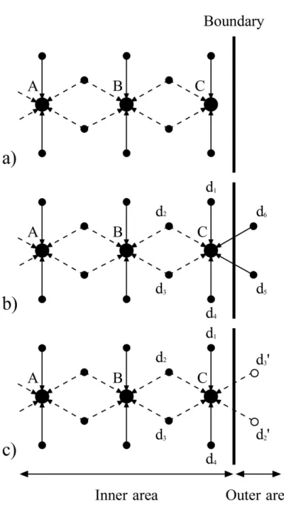
First, there is a problem that the optimal solution is not always unique because of the manner in which the objective function takes an integer value. In Kuby’s model, while the maximization of the number of firms is adopted as an objective function, there is a high possibility for the existence of multiple solutions that yield the same value for the objective function. For example, Figure 3 assumes a bounded linear market. When firm A and C have already been located as shown in Figure 3, a third firm B can be located between the two. However, this market is characterized by the presence of a small surplus that produces an excess profit. The demand that corresponds to this surplus will not support the establishment of a fourth firm. As a result, this surplus creates a corresponding degree of freedom for establishing the location of firm B. Specifically, firm B would be viable regardless of whether it was located adjacent to firm A (Figure 3-a) or at a position midway between firm A and C (Figure 3-b). Furthermore, there are other potential locations where the demand to secure the threshold is obtained. In the case of conditions that produce excess profit as in Figure 3, the above objective function will lead to the existence of multiple solutions for a firm’s location even while the

(19)

9

maximum number of firms that can enter the market is still only three.

Of course, while the maximization of the number of firms is one of the objectives of Lösch’s market area theory, an important point is that Lösch’s theory assumes maximization not only of the number of firms but also of the firm’s profits. Now, when we compare Figure 3-a and Figure 3-b, we see that the excess profit that firm B is able to secure is greater in Figure 3-b. Moreover, of all

Figure 3 Potential solutions of the locational competition by three firms

in a bounded market

The legend is the same as Figure 2.

(20)

10

potential locations available to firm B, the situation in Figure 3-b, located exactly midway between firm A and C, indicates the solution that maximizes excess profit¹. In this way, assuming that firms will act to maximize their profit and a large number of firms will appear as a result, it is desirable that they do so at points where they will be able to obtain higher profits even if the number of firms is the same. Kuby’s model lacks the setting of an objective function that reflects this behavior of individual firm that leads to the maximization of the number of firms.

The second problem with Kuby’s formulation is that when the model is applied in reality, the allocation of demand to the nearest firm is not guaranteed. Kuby (1989: 332-333) himself confirms this as a problem when actually applying the model in a number of hypothetical cases. This is because demand has no choice but to be allocated to firms who are not the nearest firms because of the priority given to the constraint that each firm satisfies the threshold rather than to the improvement of the objective function. Central place theory hypothetically assumes that consumers will use the nearest neighboring central place, and when this assumption is not based, the appropriate market area can no longer be defined. Accordingly, if we try to build an operational model that is faithful to at least the original central place theory, placing demand allocation on the nearest firm or central place represents an essential condition.

The final problem is regarding the condition of equal allocation toward equidistant nodes (this is the “indifference principle”). Although Kuby (1989) makes provision for a hypothetical area with a demand node arranged on a regular equilateral triangular grid when applying his model, this creates a possibility for the existence of multiple nearest firms at equal distances from the demand node. For example, when three firms are located at the vertices of an equilateral triangle of a certain size, the demand node at the center of the equilateral triangle will be equidistant from each firm. Therefore,

1 In Figure 3, the excess profit to be obtained by firm B corresponds to the sum of the area of the blank portion of firm B’s market-area. The problem of maximizing the area of blank portion can be solved analytically, with the answer being the situation in Figure 3-b located midway between adjacent firms.

(21)

11

theoretically, it is desirable that one third of the corresponding demand allocation should be allocated to each firm. However, when Kuby attempted to formulate the constraints to achieve equal allocation to these equidistant points, he defined the nonlinear equation that is impossible to apply the linear programming. Therefore, he adopted a linear “symmetry constraint” (Kuby 1989: 327-328) as an alternative formulation. The symmetry constraint ensures that several demand nodes equidistant from one firm become the same allocation value from that firm. Kuby is himself aware that defining this constraint is not appropriate in the formulation of an operational model for central place theory. This is because it allows for the occurrence of asymmetrical demand allocation, depending on location intervals of adjacent firms. This indifference principle problem, as described below, is critical especially when applying the model in regions where populations are not distributed uniformly.

2.3 Reformulation of Lösch’s market area theory

This section attempts to improve the Kuby’s model and to reformulate Lösch’s market area theory.

Returning to the first problem with Kuby’s model mentioned above, the reproduction of the locational equilibrium process in Lösch’s market area theory would ideally involve the setting of an objective function that considers both the maximization of the number of firms as well as the firm’s behavior to maximize their profits. Here, the situation in which the maximum number of firms is able to enter the market at the same time, as each firm is able to achieve greater profits implies the maximization of demand for the entire market. This is because if the total demand is maximized, each firm will on average be able to obtain the maximum profit. Taking Figure 3 as an example, this is represented by a situation where the total area of the ridge formed by the overlapping of the demand cones for firm A through C is maximized (Figure 3-b)².

The demand maximization was pointed out as an establishing condition for central place theory

2 However, Figure 3 assumes the case whereby the locations of firm A and C are fixed. When we hypothesize that the three firms are free to locate where they wish, total demand will be maximized when the locations of firm A and C are moved somewhat closer to the middle.

(22)

12

by Getis and Getis (1966) and was adopted by Kohsaka (1983) as an objective function when modelling the theory. Additionally, in locational competition by commercial establishments such as retail chain companies, which aim to increase their market share by developing multiple store locations, the maximization of acquisition demand is one of the purposes for which locations are used (Goodchild 1984; ReVelle 1986; Hua et al. 2011). Particularly, because it is possible to realize the distributed locations of stores and facilities when assuming the distance elasticity of demand expressed by the demand cone (Smithies 1941), the goal of demand maximization is also sometimes used to model the public facility location that considers accessibility for facility users (Holmes et al 1972; Calvo and Marks 1973; Wagner and Falkson 1975). Thus, in the sense that it can reflect the characteristics of distributed location and the behavior of firms in pursuit of profit, demand maximization may be reasonably interpreted as one of the purposes of implementing the ideals of central place theory. While Kuby (1989) himself proposes the total demand maximization as a potential alternative for the maximization of the number of firms, this is not applied in the actual model. Moreover, to my knowledge, there have been no studies that have explicitly modeled Lösch’s theory as the total demand maximization problem. Nevertheless, the total demand maximization that is premised by the demand cone is able to reproduce Lösch’s locational equilibrium process more rationally than the maximization of the number of firms.

The two remaining problems concerning Kuby’s model, namely the condition of allocating demand to the nearest firms and the condition of equal allocation to equidistant points, will need to be considered together. First, as for the former, a number of constraints for encouraging the allocation of demand to the nearest facilities have been devised in studies that have dealt with the undesirable facility location problem and the capacitated facility location problem. However, because the size of problems or allocation conditions for equidistant points can differ depending on the constraints used (e.g., Gerrard and Church 1996; Espejo et al. 2012), it is also necessary to select appropriate constraints depending on the formularization of the problem at hand. On the other hand, regarding the

(23)

13

problem of indifference principle, Gerrard and Church (1996) have demonstrated that it is possible to address the condition by adding the constraint of equal allocation to the nearest facility noted by Rojeski and ReVelle (1970). However, because this additional constraint is defined by classifying the equidistant nodes by case³, the problem tends to be large size and complicated when there are multiple equidistant nodes. To my knowledge, there is no generalized formulation for solving the indifference principle problem using a linear programming. It might be because, to begin with, the existence of more than one equidistant node has never been assumed in facility location problems for which the model is to be applied in actual regions, although this also depends on the accuracy when measuring distances. However, it is possible to define constraints of equal allocation linearly as described below. The constraint proposed for distributing demand to the nearest facility by Wagner and Falkson (1975) is adopted because there would be no inconsistency with the indifference principle.

As a result of considering the above problems, the model of Lösch’s theory in the location problem of single good is reformulated as a mixed integer programming where the total demand maximization is attempted in the following way:

maxZ = � � 𝑎_𝑖𝑞_𝑖𝑖𝑋_𝑖𝑖

𝑖∈𝑁_𝑖

𝑖 (1)

subject to:

� 𝑎𝑖 𝑖∈𝑁𝑗

𝑞_𝑖𝑖𝑋_𝑖𝑖≥ 𝑡𝑌_𝑖 ∀ 𝑗 (2)

3 For example, in the case of two equidistant nodes, a constraint is added such that the allocation value of 0.5, of 0.333 for three nodes, and so on. Thus, constraints are added for dividing the allocation value in accordance with the number of equidistant nodes.

(24)

14

� 𝑋𝑖𝑖 𝑖∈𝑁𝑖

≤ 1 ∀ 𝑖 (3)

𝑌_𝑖− 𝑋_𝑖𝑖≥ 0 ∀ 𝑖 ∈ 𝑁_𝑖, 𝑗 (4)

� 𝑋_𝑖ℎ

ℎ∈𝐹_𝑖𝑗

+ 𝑌_𝑖 ≤ 1 ∀ 𝑖, 𝑗 ∈ 𝑁_𝑖 ₍₅₎

𝑋_𝑖𝑖− 𝑋_𝑖𝑖≤ 2 − 𝑌_𝑖− 𝑌_𝑖 ∀ 𝑖, 𝑗 ∈ 𝑁_𝑖, 𝑘 ∈ 𝐸_𝑖𝑖 (6) 𝑋𝑖𝑖− 𝑋𝑖𝑖≥ 𝑌𝑖+ 𝑌𝑖− 2 ∀ 𝑖, 𝑗 ∈ 𝑁𝑖, 𝑘 ∈ 𝐸𝑖𝑖 (7)

𝑋_𝑖𝑖≥ 0 ∀ 𝑖, 𝑗 (8)

𝑌𝑖= 0,1 ∀ 𝑗 (9)

where:

a_i = population of demand node i;

qij = demand quantity from demand node i to potential firm location node j; d_ij = distance from node i to node j;

t = threshold for a firm supplying good ;

Xij = fraction of demand at node i that is supplied by a firm at node j;

1 if a firm locates at node j;

Y_j =

0 otherwise;

N_i = the set of nodes j within radius S, that is �𝑗|𝑑𝑖𝑖 ≤ 𝑆�; Nj = the set of nodes i within radius S, that is �𝑖|𝑑_𝑖𝑖 ≤ 𝑆�;

Fij = the set of potential firm location nodes h farther than node j from node i, that is

�ℎ|𝑑𝑖𝑖 < 𝑑_𝑖ℎ�;

E_ij = the set of potential firm location nodes k that are equidistant to node j from node i, that is �𝑘|𝑑𝑖𝑖 = 𝑑_𝑖𝑖, 𝑘 > 𝑗�.

(25)

15

Constraint (2) indicates that each firm satisfies threshold, with threshold t assuming a positive value. Constraint (3) prevents a demand node from over-allocating its population, and defines that demands at node i are equal to zero if the distance between nodes i and j is beyond the radius S which represents the upper limit of the range of a good. Constraint (4) states that demands at node i can only be assigned to a firm at node j if a firm is located at node j (this is the “self-assignment constraint”).

Constraint (5) is the closest assignment constraint introduced by Wagner and Falkson (1975), and constraints (6) and (7) guarantee the indifference principle. Specifically, in the case of a firm located at node j (i.e., when Yj = 1), all demand allocations from demand node i toward potential firm location node h become zero according to constraint (5), indirectly encouraging the allocation of demand to the nearest node. Then, by virtue of constraints (6) and (7), in the case that there are firms located at nodes j and k, which are equidistant from point i (i.e., when Yj = Yk = 1), equal allocation is realized because 𝑋_𝑖𝑖 ≤ 𝑋_𝑖𝑖 ≤ 𝑋_𝑖𝑖and 𝑋_𝑖𝑖 = 𝑋_𝑖𝑖 hold true. In the case that there is no or only one firm at nodes j and k, then both constraints (4) and (8) represents that either 0 ≤ 𝑋𝑖𝑖 ≤ 1 or 𝑋𝑖𝑖 = 0 when taking X_ij as an example.

Here, we need to define the amount of demand qij from node i to node j on the basis of the concept of demand cone. While Kuby (1989) sets four parameters of the price of good, the transportation rate per unit of distance, the slope of the demand curve (distance elasticity), and the maximum demand, ultimately we only need consider two parameters of the maximum demand without the addition of transportation costs and the elasticity of demand per unit of distance.

Accordingly, this paper assumes a simple linear relationship between distance and demand⁴ as shown in Figure 1, and defines the quantity of demand as follows:

4 It is, of course, possible to define a non-linear function, but such a function would still have the same properties in the sense that demand decreases monotonically with respect to distance.

(26)

16 𝑞𝑖𝑖 = �𝑄 − 𝛽𝑑𝑖𝑖 𝑑𝑖𝑖 ≤ 𝑆

0 𝑑_𝑖𝑖 > 𝑆 ⁽¹⁰⁾

where Q represents the maximum demand and β the distance elasticity of demand, with Q > 0 and 𝛽 ≥ 0. Incidentally, when β is a positive, the theoretical upper limit S of the range of a good can be represented as Q/β.

2.4 Setting a hypothetical area

It is well known that Lösch assumed a hypothetical plain distributed with regular, discrete settlements as the space in which firms would be located (Lösch 1954: 114-116). Storbeck (1988, 1990) and Kuby (1989), who have attempted to model central place theory, have also used uniform lattice networks as a hypothetical area for applying the model, attempting to derive a theoretical central place system with a central places or firms located at equal intervals. Similarly, this chapter sets a hypothetical area consisting of a regular and discrete point distribution.

However, problems tend to be large size in the model detailed in the previous section, especially in constraints (4) through (7), because the number of constraint formulae increases significantly with an increase in the number of nodes. This tendency is particularly notable when using a two-dimensional market as a hypothetical area. Therefore, this chapter attempts to apply the model chiefly to the hypothetical area of a linear market in which problems can be kept comparatively small and it remains possible to obtain efficient solutions, and then expands the discussion to a two-dimensional market on the basis of the findings obtained.

The hypothetical area of the linear market used in this chapter, as shown in Figure 4, includes 61 nodes with integer values of 0 through 60 as coordinate values along the x-axis, regularly distributed in a straight line. Each node is simultaneously a demand node and a potential firm location node, and the distance between nodes is measured using Euclidean distance. The population a_i on the demand

(27)

17

node is assumed to be distributed in two patterns, namely uniformly and non-uniformly (Figure 4). In the former case, the population for all demand nodes is taken to be 100, while in the latter the population is distributed according to Clark’s (1951) model presented below when the market center is a node where x coordinate value is 30:

𝑎𝑖 = 𝑝𝑒^−𝑏𝑑^𝑖 ⁽¹¹⁾

where p is a market center population, b is the decline rate of population, and di is the distance from the market center to node i. Specifically, p = 200, b = 0.05. Incidentally, the total population of the 61 demand nodes obtained by Equation (11) is 6,261, which is comparable with the total population of 6,100 when the population is uniformly distributed.

The reason for adopting Clark’s model, known as the law of urban population density, is that Lösch’s market area theory can be regarded as an alternative theory of tertiary activity on an intra-urban scale (Beavon 1977), as well as that examines to validate what the “cobweb-like”

Figure 4 Hypothetical linear market and uniform and non-uniform

distributions of population

(28)

18

economic landscape (Parr 1973: 192) introduced by Isard (1956: 272) when their population density is as low as that of the surrounding area.

In the development of their theories, both Christaller and Lösch assumed the continuous and unbounded plain as a space for the location of their central places. However, we have no choice but to apply our model to a finite space of discrete nodes where the number of nodes is limited. The application of the model to a finite space produces distortions, especially in the regularity of the location of firms near the boundary of hypothetical area (Kuby 1989). Let us examine this problem in more detail using Figure 5, which posits a uniform population distribution.

Figure 5-a represents an example of a hypothetical area closed by boundaries, firm C, who is located near the boundary, being unable to obtain demand allocation from outside the area, is only able to obtain a smaller quantity of demand compared to firms A and B. Although theoretically the three firms locates at regular intervals, if it is estimated that the quantity of demand that firm C can acquire is less than threshold, then firm C will not enter the market or will seek elsewhere at a node where the threshold can be satisfied. Either way, the change in the demand allocation pattern will create an imbalance in acquisition demand for each firm such that the regularity of the location will be lost.

To deal with this boundary problem⁵, it is necessary to consider how to assume the presence of demand allocation outside the region. Kuby (1989) enabled demand allocation from outside the region by separating his hypothetical area into an inner area comprising demand nodes and potential firm location nodes and an outer area comprising only demand nodes where firms could not be located. However, to overcome the above problem, simply setting an outer area is not sufficient.

For example, Figure 5-b indicates the presence of demand allocation to firm C from demand nodes d₅ and d₆, which are placed in the outer area. Under normal circumstances, the demand

5 This problem is similar to so-called “edge effects” in the point pattern analysis (Bailey and Gatrell 1995: 90).

(29)

19

Figure 5 Demand allocation pattern near the boundary

Solid line represents to allocate all population at demand node to firm location and dashed line is half allocation.

(30)

20

allocation from these two nodes should be shared between firm C and the adjacent firm, as can be surmised from firm B’s demand allocation pattern. However, because competing firms cannot be located in the outer area, firm C is able to have a monopoly over the demand allocation from the outer area. In this way, as the tendency to be located near boundaries with advantageous demand acquisition reinforces, this ultimately results in a number of firms different from that predicted by the theory and the occurrence of irregularities in the location pattern.

Kuby’s symmetry constraints mentioned above are also a device for making a demand allocation from the outer area equivalent to that from the inner area. However, if nodes d1 through d6 in Figure 5-b are all equidistant from the location of firm C, this causes problems for the symmetry constraints.

This is because while it is desirable for nodes d2, d3, d5, and d6 to have symmetrical allocation values of 1/2 and all demand from nodes d1 and d4 should be allocated to firm C. Thus, it is possible to become different allocation values even if these nodes are equidistant from the same firm.

Therefore, the following approach to the boundary problem is taken. Namely, “to add virtual demand allocation for demand nodes for which there is no point symmetry, when assuming potential firm location nodes as centers of symmetry.” Using Figure 5-c as a specific example, now, for node d1, node d4 exists in the inner area to provide point symmetry with respect to the location of firm C.

However, the locations that would provide point symmetry for nodes d2 and d3 correspond to the outer area and do not exist in the inner area. Thus, to account for these points d2 and d3, which lack point symmetry locations, we will posit the existence of virtual points d2'

and d3'

. Thereafter, we will be able to add the demand allocations to firm C for an equivalent value of the demand allocations from nodes d₂ and d₃.

In fact, we are now able to deal with constraint (2) above, which relates to the threshold condition, as follows:

(31)

21

� 𝑎𝑖 𝑖∈𝑁𝑗

𝑞𝑖𝑖𝑋𝑖𝑖 + � 𝑎𝑖 𝑖∈𝑁𝑗∩𝑂𝑗

𝑞𝑖𝑖𝑋𝑖𝑖 ≥ 𝑡𝑌𝑖 ∀ 𝑗 ₍₁₂₎

where Oj is the set of demand nodes i corresponding to the potential firm location node j for which no point symmetry locations exist. That is, when point symmetry locations exist, then we include the usual demand allocation. When point symmetry locations do not exist, then we include twice the usual demand allocation.

Herein, the condition of point symmetry for demand allocation described above will be referred to for the time being as the “mirror effect.” Application of the mirror effect will be limited to the threshold condition in constraint (12), and we will not introduce it into the objective function (1) that maximizes the total demand. This is because the tendency to be located near boundary areas is fostered similar to Figuire 5-b when the demand allocation from outer area is considered as an optimization variable.

2.5 Solving the total demand maximization problem

In applying the model to the linear market in Figure 4⁶, we set the maximum demand Q = 10 and the distance elasticity of demand β = 0.8 in Equation (10). Additionally, the upper limit of the range of a good is set to S = 10. When β = 1, this is consistent with the theoretical range of a good (Q/β), but in that case demand would fall to 0 at a demand node ten units apart from the firm location, and demand allocation becomes meaningless. Accordingly, our parameters have been adjusted so that demand does not fall to 0 inside the demand cone.

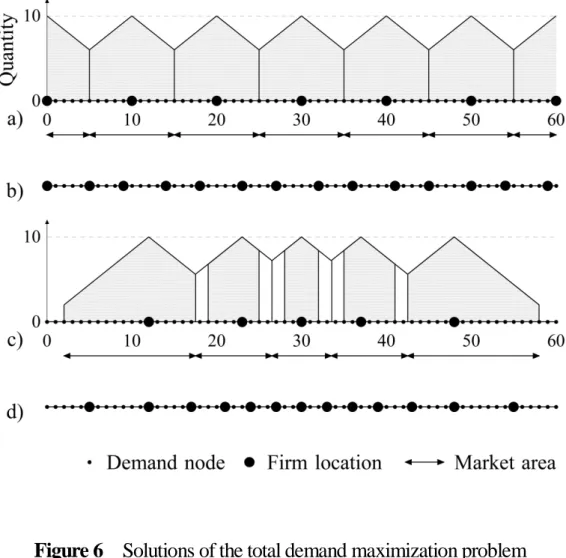
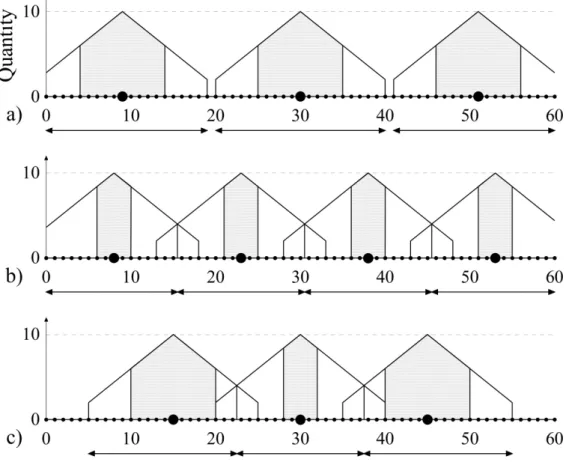
Figure 6 shows the results of applying the model when t = 8,000 and t = 4,000. From Figure 6-a, which has a uniform population distribution and t = 8,000, we find seven firms located at equal

6 In this paper, all problems are solved using NUOPT ver.15.1.0 by NTT DATA Mathematical Systems Inc.

(32)

22

intervals. The total demand quantity of each firm is exactly 8,000 that is sum of demand at nodes within a radius of four units from each firm location and demand at nodes divided into two among adjacent firms. Accordingly, when each firm is located next to another while maintaining a market area with a radius of five units, the number of firms able to enter the market and the total demand of the entire market is maximized with each firm able to obtain only a normal profit. In Figure 6-a, while there are firms located at both ends of the linear market at the x-coordinates 0 and 60, these firms are unable to meet the threshold using only demand from within the market. However, by employing the

Figure 6 Solutions of the total demand maximization problem

in a linear market

Shaded area corresponds to the quantity of threshold. Demand cones are omitted in b) and d).

(33)

23

mirror effect from constraint (12), these firms will be able to secure the threshold by accepting demand allocation from a virtual outer area.

Even though the population distribution is uniform, it remains somewhat lacking in regularity for t

= 4,000 (Figure 6-b). This is because, under the values we set earlier for the maximum demand Q = 10 and the distance elasticity of demand β = 0.8, there will be no solution that would be exactly equal to 4,000 for each firm, which results in the production of excess profit, leading the market area to become asymmetrical⁷. If we assume a discrete point distribution, then this presents us with a problem that we will have to somehow overcome.

This asymmetry of market area also arises in the event of a non-uniform population distribution.

Figure 6-c shows the results of the case where threshold is set to 8,000 for a non-uniform population distribution. When this is compared against a case with a uniform population distribution (Figure 6-a), we see that the market area size varies significantly depending on location, producing asymmetry. In other words, while it is possible to meet the threshold within a comparatively confined market area in the vicinity of market centers with dense populations, a much wider market area is needed to acquire the demand satisfied the threshold in areas with a sparse population distribution. Because the breadth of distance between firm locations is determined in response to population distribution, drawing boundaries between market areas for adjacent firms in a linear market could cause the development of market areas characterized by left–right asymmetry. This tendency will be similar in the case where threshold is set to 4,000 for a non-uniform population distribution (Figure 6-d). As stated above, using the symmetry constraint used by Kuby (1989) implies that nodes that are equidistant from a firm location have the same demand allocation value, thus preventing the emergence of the asymmetric market areas.

From Figure 6-c, we see that in addition to excess profits occurring for firms in the vicinity of

7 Specifically, the solutions that yield values closest to 4,000 are 3,680 and 4,100. In the latter case, which satisfies the threshold, the allocation value takes a left–right asymmetry at demand nodes at a radius of two units from the firm location.

(34)

24

market centers, there are also demand nodes not included in the demand cones toward both edges of the market. The former is the effect of a discrete point distribution. If the market were a continuous space, firms would likely be located even more closely together. The latter is the result of the coverage condition of a good as shown in constraint (3). As opposed to Christaller’s central place theory, which covers all demand nodes inside the upper limit of the range of a good (that is “mandatory coverage”), Lösch’s market area theory prioritizes firm’s acquisition of profit. As a result, it is possible that uncovered area will appear in areas with low demand.

Application of the model to a non-uniform population distribution is similar to the case wherein density conversion is employed for deforming the hexagonal networks of central places in response to demand allocation; cartograms (Getis 1963) and map transformation techniques (Rushton 1972;

Sugiura 1991) are a few such examples. Then, imagining a situation where we rotate the linear market, expanding it as a two-dimensional market, we can infer the bias pattern of market area networks in the case of non-uniform population distribution of Isard (1956).

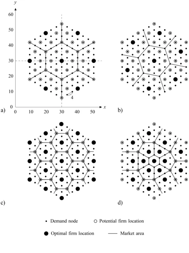
Although there is a risk of large size problems occurring when the model is applied to a two-dimensional market, let us examine below the possibility of applying the model using a relatively small size two-dimensional market as a hypothetical area. The hypothetical area is a discrete space of 127 demand nodes and 43 potential firm location nodes on a regular equilateral triangular grid as shown in Figure 7. Note that not all demand nodes are potential firm location nodes for the following two reasons: (1) to reduce the size of the problem and (2) to consider the influence of blank areas where there is no demand between nodes⁸.

When applying the model, because the nearest distance between nodes in Figure 7 is four units

8 When assuming a discrete point distribution, the fact that there is a possibility of “gaps” occurring in the supply of a good between nodes implies that our hypothetical area would not fulfill its role as a continuous virtual plane. I have addressed this problem by placing demand nodes separately from potential firm location nodes. For a closer discussion, see Ishizaki (1992). Note that there are some cases in which it is possible to examine central place systems when uncovered areas occur (Church and Bell 1990).

(35)

25

Figure 7

Solutions of the total demand maximization problem

in a plane market

(36)

26

and considering the number of nodes, the following parameters have been set. Namely, the maximum demand Q = 10, the distance elasticity of demand β = 0.5, and the upper limit of the range of a good S

= 16. As with the linear market, the population distribution is such that all nodes have a population of 100 in uniform distributions, while the non-uniform distributions of population have been calculated on the basis of Equation (11). Specifically, setting one node where x- and y-coordinate values are 30 in Figure 7 as market center, the parameters for Equation (11) have been set to p = 300 and b = 0.08.

As a result, the aggregate population for 127 demand nodes is 12,013, which is approximately the equivalent of a population of 12,700 in the uniform population distribution case. In addition, to facilitate the comparison of the model’s results for different population distributions and threshold conditions, the constraint that at least one firm must be located in a market center has been added to the model.

Figures 7-a through c represent the results of applying the model for uniform populations with respective thresholds of t = 16,000, t = 14,000, and t = 6,000, while Figure 7-d shows the result for a non-uniform population with a threshold of t = 5,000. Summarizing the findings obtained from these results, we can confirm the following among other things: (1) as Beavon (1977) has summarized for Lösch’s theory for uniform population distributions, regular hexagonal networks of various sizes are formed because the number of demand nodes included in a market area is different according to the threshold value, and that (2) as indicated by Isard (1956), for non-uniform population distributions, market area networks emerge in which the hexagonal structure is distorted.

As can be seen by comparing Figure 7-a and Figure 7-b, the derivation of market area networks of different sizes, even for the same number of firms, is the result of the fact that an objective function of the model is not the maximization of the number of firms but the maximization of total demand. In addition, the mirror effect in Equation (12) and the condition of the equal allocation of demand in constraints (6) and (7) result in the realization of a pattern whereby firms are located at regular intervals while securing a minimum market area that yields normal profit. Furthermore, in the case of

(37)

27

a non-uniform population distribution, we can see that it corresponds to the formation of more realistic (if more complex) market area networks, as in the case of nodes allocated equally to four equidistant firms.

From the above, we may regard the model demonstrated in this chapter as a model that reliably reproduces the locational principle and preconditions in Lösch’s market area theory. Moreover, this model will be considered as an operational model that enables the derivations of theoretical location patterns even under various real-world conditions.

2.6 Developing the total profit maximization problem

As described above, in Lösch’s market area theory, which considers locational equilibrium to be the result of perfect competition and free entry of firms into the market, the firm will be unable to obtain anything other than normal profit. However, in reality, according to the changes of population distribution, prices, and production costs in the market, it is possible that excess profits will begin to accrue after locating firms once or that a firm will only be able to achieve demand that falls below the threshold. To begin with, the situation where no firm is able to obtain excess profit is extremely unrealistic. Conversely, what would be the most profitable situation for a firm? This would be when a firm is able to secure all excess profits included in the market area of radius S within the demand cone shown in Figure 1.

Figure 2-a represents a situation in which firms A and B participate while securing maximum profit. If we assume this linear market to extend infinitely, then each firm will not only locate without overlapping a market area of radius S, but also will ensure that all demands are captured in the market.

In contrast to “the total demand maximization problem”, in which each firm is located as close to one another as possible on the condition that a normal profit can be obtained, this can be considered as

“the total profit maximization problem” (Hansen and Thisse 1977). In this case, all firms participating in the market are able to obtain maximum excess profit.

(38)

28

In the example given in Figure 2-a, the total profit is represented by the total area of blank parts. In other words, it is simply the total area that is obtained by subtracting the total area of shaded parts as two firm’s thresholds from the total area under the ridge as the total demand. Accordingly, the total profit maximization problem can be formulated by correcting the objective function (1) to the following equation and by using constraints (2) through (9) without modifying them:

maxZ = � � 𝑎_𝑖𝑞_𝑖𝑖𝑋_𝑖𝑖

𝑖∈𝑁_𝑖 𝑖

− � 𝑡𝑌_𝑖

𝑖 (13)

Here, let us apply the total profit maximization problem to the linear market of the hypothetical area in Figure 4. Our parameters, just as with Figure 6, will be maximum demand Q = 10, distance elasticity of demand β = 0.8, and the upper limit of the range of a good S = 10. Additionally, the mirror effect is applied by using constraint (12) instead of constraint (2). Figures 8-a and 8-b represent the results of applying the model to uniform populations with respective thresholds of t = 8,000 and t

= 4,000, while Figure 8-c shows the result for a non-uniform population with a threshold of t = 8,000.

From Figure 8-a, we find that each firm has a monopoly over a distance of ten units that represents the maximum radius of the demand cone, with three firms participating in the market located at equal intervals. Hence, under normal circumstances, maximum excess profit will be obtained for each firm when they are located without any overlap in the demand cone. However, when threshold is set to 4,000, by increasing the number of firms participating in the market, the interval between firm locations is narrowed, necessarily leading to a subdivision of the market area (Figure 8-b).

Given infinite space, the fourth firm would enter outside area, as shown in Figure 8-a, and each firm would be able to earn even greater excess profit without any mutual market area interference.

However, even considering the mirror effect expressed in constraint (12) into account, the linear

(39)

29

market of our hypothetical area is not infinite. Accordingly, insofar as we are considering a finite space, the addition of a firm inside a limited market as in Figure 8-b can sometimes lead to the occurrence of a rise in total overall profits depending on threshold values.

In addition, even in the case of a non-uniform population distribution, demand cone overlap can still be confirmed (Figure 8-c). This is because firms intend to be located in a densely populated area that is more advantageous for earning profit than the surrounding area with little prospective demand.

As a result, even if the market areas of radius S are partially overlapped between firms, the total profit is maximized in the entire market. Therefore, in the case of a non-uniform population distribution,

Figure 8 Solutions of the total profit maximization problem

in a linear market

The legend is the same as Figure 6.

(40)

30

there is a conceivable possibility that demand cones will overlap regardless of whether the space is finite or infinite.

In contrast to the total demand maximization problem (Figure 6) which seeks to maximize the number of firms, there are fewer firm locations in the total profit maximization problem. The total profit maximization problem represents an antithetical model in the sense that it supplies a good by having as few locations as possible.

2.7 Extension of the model using multiobjective programming

If Lösch’s market area theory is regarded as the total demand maximization problem on the unrealistic assumption of perfect and free competition, then we will be forced to admit that the total profit maximization problem is also unrealistic in the same way. This is because it is difficult to imagine that firms will make efforts together with one another to secure maximum excess profit without encroaching on each other’s areas, as shown in Figure 2-a. A situation such as the one shown in Figure 2-a is limited to an extreme case, for example, when a market is monopolized by only one company (Ghosh and Harche 1993).

A solution between the two extremes of the total demand maximization and the total profit maximization is realistically conceivable. In other words, a situation in which a certain degree of excess profit is to be expected is plausible. The method for simultaneously optimizing such multiple and competing objectives is known as multiobjective programming (Cohon 1978). Multiobjective programming typically involves the use of a weighting method that combines multiple objective functions by applying a weighting to each individual objective and then adjusting the weighting minutely to derive several eclectic non-inferior solutions (Pareto optimal solutions).

Therefore, the extended model in which two objectives are integrated can be formulated as follows using multiobjective programming by substituting Z1 for the right-hand side of objective function (1), which represents the total demand, and Z₂ for the right-hand side of objective function

(41)

31 (13), which represents the total profit:

maxZ = (1 − 𝑤)𝑍₁+ 𝑤𝑍₂ ⁽¹⁴⁾

where w is a weight that takes a value of 0 ≤ 𝑤 ≤ 1. Namely, when w = 0, the objective function (14) represents the total demand maximization problem, and when w = 1 it equivalent to the total profit maximization problem. Moreover, because eclectic solutions for both can be obtained when 0 < 𝑤 < 1.

Here, let us apply the extended model to the hypothetical area in Figure 4. To avoid complication, we will demonstrate only the solution for a uniform population distribution where threshold t = 8,000.

Note that our parameters will be as they have been thus far, with maximum demand Q = 10, distance elasticity of demand β = 0.8, and the upper limit of the range of a good S = 10. In addition, the constraints will be according to constraints (3) through (9), with the mirror effect applied by adopting constraint (12). Weighting w is varied in increments of 0.01.

Table 1 lists five non-inferior solutions obtained by changing the weighting w. Of these solutions, Solution A corresponds to the solution to the total demand maximization problem (Figure 6-a), whereas Solution E corresponds to a solution for the total profit maximization problem (Figure 8-a).

Among the objective functions, there will be cases when total profit takes a negative value, because while extrinsic demand will be added to the threshold condition by the mirror effect of constraint (12), the demand in question will not be reflected in the objective function. Accordingly, a negative total profit does not necessarily mean that the threshold is not satisfied.

By observing the transition of the two objective function values in Table 1, we can see that there is a trade-off relationship between the two objectives. In multiobjective programming, an absolutely optimal solution that is simultaneously optimal for multiple objectives generally does not exist. Hence, on the basis of the variations in each objective function value, we turn to weigh the compromise

(42)

32

alternative of our non-inferior solutions. Accordingly, rather than leading us to a unique optimal solution, multiobjective programming offers a richly flexible model in the sense that it seeks out solutions interactively from among many competing objectives.

Of five non-inferior solutions in Table 1, Figure 9 shows the results of Solution C situated middle solution between the two objectives of total demand maximization and total profit maximization. All five solutions show a trend for forms to be located at equal intervals, and solution C is no exception.

Total demand (Z₁) Total profit (Z₂)

A 0.00～0.04 49,000 -7,000 7

B 0.05～0.30 48,600 600 6

C 0.31～0.46 46,120 6,120 5

D 0.47～0.78 42,440 10,440 4

E 0.79～1.00 36,200 12,200 3

Solution w Objectives Number of

firms Table 1 Non-inferior solutions of the extended model

for single good

Figure 9 Locational pattern of non-inferior Solution C in Table 1 The legend is the same as Figure 6.

(43)

33

We might go so far as to say that the results shown in Figure 9, which are similar to neither Figure 6-a nor Figure 8-a, illustrate the situation whereby each firm is able to earn moderate excess profit.

Ultimately, the differences between five non-inferior solutions depend on the number of established firms. The weight w of objective functions in multiobjective programming is a relative indicator for deriving multiple non-inferior solutions, and the value of the weighting itself does not necessarily have any meaning. Although each of non-inferior solutions shown in Table 1 appears for a certain range of values of weight w, the objective function values Z₁ and Z₂ remain constant within that range. In other words, the model represented by objective function (14) may be thought of as a model that variably captures the number of firm locations while extending Lösch’s model ultimately to the maximum number of firms entering into the market.

(44)

34