A study about the improvement of the interpretative accuracy of compound geophysical explorations by self-organizing maps

A study about the improvement of the interpretative accuracy of compound

geophysical explorations by self‑organizing maps

著者 Yamamoto Tatsuru, Kusumi Harushige, Yamamoto Tsuyoshi, Tsuji Takeshi

journal or

publication title

Proceeding of EIT‑JSCE Symposium on

Engineering for Geo‑Hazards:Earthquakes and Landslides‑for Surface and Subsurface

Structures

year 2010‑09‑06

URL http://hdl.handle.net/10112/5636

A study about the improvement of the interpretative accuracy of compound geophysical explorations

by self-organizing maps

Tatsuru Yamamoto

, Harushige Kusumi

, Tsuyoshi Yamamoto

and Takeshi Tsuji

1

Graduate school of Kansai University E-mail : [email protected]

2

President, Kansai University E-mai

3

E-mail : [email protected]

Planning Dept., Kinki Regional Development Bureau, Ministry of Land, Infrastructure, Transport and Tourism

4

Environment and Resource System Engineering, Kyoto University E-mail : [email protected]

ABSTRACT: In Japan, in the high economic growth period in 1960’s, a great number of slopes were formed to construct many roads. Now, the slopes have been aging, it is important to estimate the health of the aging slope and maintain slopes effectually. So, in situs, we usually carry out seismic wave method, surface wave method, electric method, electromagnetic wave method, frequency domain electromagnetic method and so on. However, there is not the technique to compound and interpret the result of each geophysical exploration in a numerical formula of the engineering now. Therefore, we notice to self-organizing maps (SOM) used widely in a field of the information processing engineering, and tried to interpret multidimensional data by integrating. In this paper, we classified the ground property by self-organizing maps. The classification result is relatively conformal with boring data. Therefore, it is recognized that it can be used to improve the interpretative accuracy of compound geophysical explorations. And, it can be shown that this technique is effective to estimate of the ground property of the aging slope.

1. INTRODUCTION

In the investigation of the soundness of the aging slope, the method that attracts attentions is to make an overall evaluation by using two or more geophysical explorations. However, the technique for interpreting two or more geophysical overall explorations at present is not established, and it is a current state that an advanced judgment based on the engineer's exclusive knowledge and experience is demanded, and there is a possibility that the difference is caused in the interpretation of the geophysical exploration.

Therefore, in this paper, we used SOM which is widely used in the field of information processing engineering and clustered the data of two or more geophysical explorations measured in situ clustered, and proposed the technique for overall interpretation. As a result of the classification by SOM, it is related to RQD, the rock kind and the rock class division that became clear in the boring investigation. Therefore, it was able to show that this method was effective for the improvement of the interpretative accuracy of compound geophysical explorations to understand rock properties of the aging slope.

2. GEOLOGICAL CONDITIONS IN THE RESEARCH SITE

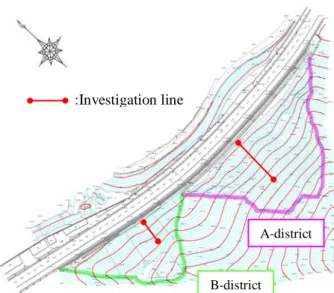
An analytical object in this research is a cutting ground slope along the national road No.9 in Omi district in Fukuchiyama City in Kyoto in Japan.

Figure.1 shows topographic features of the slope, and Figure.2 shows the view of the shotcrete slope (A-district) and Figure.3 shows the view of the non-support slope (B-district). These are near the south of the national road, and comparatively large-scale slopes of about 200m in length and about 50m in height. The shotcrete slope (A-district) is distributed in the eastern part of the slope, and the non-support slope (B-district) is distributed in the western part of it. There are a lot of cracks on the surface on the slope with shotcrete (A-district) due to aging, and a lot of vegetation from the cracks and the swells are seen. The non-support slope (B-district) is a naked ground slope, and there is hardly a big transformation that can be seen.

Geological features are in Tanba strata at Triassic

in the Mesozoic-Jurassic Period, and they are

chiefly composed of sandstone layer, a sandstone

shale alternation of strata, and a green rock layer.

Figure.1 Topographic features of the slope

Figure.2 View of the shotcrete slope (A-district)

Figure.3 View of the non-support slope (B-district)

3. ANALYTICAL METHOD

(1) Compound geophysical explorations

The geophysical explorations executed in situ are the seismic tomography method, the surface wave method, the electromagnetic tomography method, and the frequency domain electromagnetic method (FDEM). In both A district and B district, they were executed four times in total in summer and winter of 2008 and 2009. However, at the A-district, geophysical data is not sensitive enough, influenced by the shotcrete and metal bodies behind the shotcrete. Therefore, the result of the B-district was used for the evaluation by SOM. And, we

compared the datum of the same period of the summer in 2008 and 2009

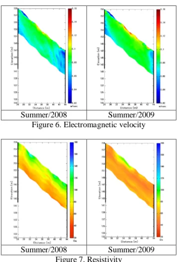
Figure 4 shows the P wave velocity obtained by the seismic tomography method. This shows the tendency that the speed transmitted in the ground quickens as depth becomes deep. Figure-5 shows the S wave velocity obtained by the surface wave method. Figure-5 shows the S wave velocity obtained by the surface wave method. In a local low-speed region, it is surmisable that there is the change in the ground physical properties. Figure-6 shows the electromagnetic velocity obtained by the electromagnetic tomography method. It is shown the high percentage of water content if the electromagnetic velocity is slow, and the low percentage of water content if it is fast because the electromagnetic velocity depends on the water content in the ground. Figure-7 shows the resistivity obtained by FDEM. This is obtained from the second magnetic field intensity caused when faradic is generated by the first magnetic field intensity and the first magnetic field intensity generated while changing the frequency from the exploration equipment in the ground. Moreover, because it is possible to make a simple measurement compared with other methods, this method is promising in the investigation on the slope of the rapid inclination.

Summer/2008 Summer/2009

Figure 4. P-wave velocity

Summer/2008 Summer/2009

Figure 5. S-wave velocity

A-district

B-district

:Investigation line

Summer/2008 Summer/2009 Figure 6. Electromagnetic velocity

Summer/2008 Summer/2009

Figure 7. Resistivity (2) Self-organizing maps

Self-organizing maps is a kind of the neural net work developed by professor Kohonen of Helsinki university. This has the feature in which the input data of higher dimension data can be mapped to SOM plane of two dimensions in proportion to the degree of similarity. In a word, data with a different feature has the feature in which the map arranged at a position away can be made so that data with a similar feature is near. As a standard by which the degree of similarity is shown, Euclidean distance between data is used. It is judged that two data which this Euclidean distance is near looks like.

Moreover, SOM can cluster without the preliminary knowledge of data. The basis of the algorithm of SOM is shown in Figure.8.

First of all, the two-dimensional map is initialized. An individual neuron with the same dimension as the input vector is arranged in two dimension SOM plane at random besides the input vector.

Secondarily, it searches for the champion vector.

The champion vector is the one when Euclidean distance that shows the degree of similarity shown in the expression (1) is minimized. In a word, it looks for the most similar reference vector to the input vector.

[ ]

1

∑

−

=

−

=

k

jk ik j

i

m x m

x

d (1)

Here, x

: the input vector, m

: the reference vector Thirdly, according to the expression (2) shown below, the champion vector and the circumference unit near the champion vector learn the input vector.

The neighborhood size is reduced as the learning progresses.

[ ^{( ) ( )} ]

) ( ) ( ) 1

( t m t h t x t m t

m

+ =

+

−

⁽²⁾

Here, m

(t) : information processing ability, h

(t) : the update rate, x(t) : the input vector.

The update rate is a ratio in which the champion vector and the vector near the champion vector is updated, and it is changed in proportion to the learn frequency as shown in expression (3).

 

 



 −

= 2 ( )

) exp (

) ( )

(

2

t t t d

t h

α σ ⁽³⁾

Here, α (t) : the learning coefficient, d(t) : the distance from the champion vector, σ(t) : the learning radius from the champion vector.

The learning coefficient and the learning radius from the champion vector are shown in the expression (4) and the expression (5). These

unspread the vector of the neuron by setting them to decrease with an increase in the learning frequency.

 

 

  −

= T

t ) 1 t ( α

α ⁽⁴⁾

 

 

  −

= T

t ) 1 t ( σ

σ ⁽⁵⁾

Here, α

: the initial value of the learning coefficient, σ

: the initial value of the learning radius, t : the learning frequency, T : All learning frequency

Fourthly, the SOM map is clustered. Repeating the search and the study of the vector a number of times, the vector with high similarity is arranged on the SOM map. And, considering those Euclidean distances makes it possible to classify the SOM map.

Finally, the input vectors classifies. By applying

the input vectors to the clustering SOM map, it is

understandable which class the input vectors are

classified.

(1) Initialization of SOM map

(2) Search for champion vector

(3) Learning of champion vector and unit near it

(4) Clustering of SOM map

(5) Class separation of input vector Figure.8 The basis of the algorithm of SOM (3) Adjustment of input geophysical data

As for the P wave velocity section, the S wave velocity section, the resistivity section, and the electromagnetic velocity section used by this research, the method of acquiring geophysical data is different. Therefore, the length of the investigation line, the exploration depth, and the sampling cell interval acquired are different. Then, we standardized the geophysical data interval with the interpolation of each geophysical data, and the cell interval, and unified the acquired geophysical exploration data as 0.5m. The geophysical properties distributions acquired by each geophysical exploration shown from Figure.4 to Figure.7 have already been standardized. In addition, each geophysical data to input to SOM is different in the range of the maximum value and minimum value and the degree of variance value.

Geophysical data that variance value is small reduces a relative influence on the output result by SOM. Therefore, we conducted a linear standardization to make the variance value one so that the importance of each data becomes equal.

(4) Classification result by SOM

The SOM map that studies each input geophysical data is shown in Figure.7 and Figure.8.

The SOM map is not the one that shows the vertical direction and the horizontal direction of two dimension plane but only arranges a similar vector in neighborhood. Therefore, it is necessary to read how the geophysical values are distributed in the SOM map, and it is also necessary to classify the geophysical values in the SOM map, considering Euclidean distance that shows the degree of similarity between geophysical data. In this research, the boundary of the cluster was set at the position where Euclidean distance between datum that belonged to each neuron in the SOM map was far (the degree of similarity was small), and the number of clusters was 3. Data that belonged on the boundary of the cluster was set as cluster 4 that was the area where the cluster was not able to be specified for cluster 1 - cluster 3. The result of clustering by considering the SOM map is shown from Figure.9 to Figure.12, and Table.1 and Table.2 show the relative amount of each geophysical data.

The result of the boring investigation comparison is shown in Figure.13 and Figure.14.

In the classification result at both time of the

summer of 2008 and 2009 of Figure.13 and

Figure.14, the cluster 3 is corresponding to the area

that RQD is zero. The cluster 3 is in the rock class

division between D class and E class. In addition, it

is thought that the cluster 3 is an area where the

influence of weathering is the strongest because the

cluster 3 is corresponding to the weathering shale

layer estimated by the boring investigation. The

change of physical properties of the weathering

green rock can be presumable in the cluster 2 and

the cluster 1, because they are in the area in the

weathering green rock layer presumed by the boring

investigation. As shown in Figure.13 and Figure.14,

the characteristic difference cluster 2 and cluster 1

is that there is a change in the area where the S

wave velocity, electromagnetic velocity, and

resistivity are low in the cluster 2, while the

distribution of each physical value shows an almost

similar tendency in the cluster 1. This is thought to

be some error of the measurement and the change

of the weather condition. Because of this, it is

thought that some changes took place in the

distribution of the cluster 2 in the classification

result in summer of 2008 and 2009. However, it can

be said that the quality of the rock in the cluster 1 is

comparatively better than that in the cluster 2 by

comparing the rock class division by the boring

investigation, since it is understood to belong from

D class to CM class roughly in the cluster 2, and to

belong from CM class to B class roughly in the

cluster 1. As for the cluster 4 set as a boundary of the cluster there are some area where cluster 4 is locally distributed in the cluster 1, cluster 2 and cluster 3. This shows the possibility of meaning some feature of some rock properties in the area of the cluster 4.

Summer/2008 Summer/2009

Figure.9 SOM map of the P-wave velocity

Summer/2008 Summer/2009

Figure.10 SOM map of the S-wave velocity

Summer/2008 Summer/2009

Figure.11 SOM map of the electromagnetic velocity

Summer/2008 Summer/2009

Figure.12 SOM map of the resistivity

Table.1 The relative amount of each geophysical data (Summer/2008)

Cluster 1

Cluster 2

Cluster 3

P-wave velocity *** ** *

S-wave velocity *** * **

Electromagnetic

velocity ** * ***

Resistivity * ** ***

Table.2 The relative amount of each geophysical data (Summer/2009)

Cluster 1

Cluster 2

Cluster 3

P-wave velocity *** ** *

S-wave velocity *** * **

Electromagnetic

velocity ** ** ***

Resistivity ** * ***

Figure.13 Classification result of Summer/2008

Figure.14 Classification result of Summer/2009 4. CONCLUSION

In this research, the geophysical data was characterized and classified to three clusters by SOM that widely used in the field of information processing engineering to interpret the result of two or more geophysical explorations comprehensively.

The opinions obtained from this research are shown as follows.

1) By using four kinds of different dimensional geophysical value (the P wave velocity, the S wave velocity, the electromagnetic velocity, and the resistivity) that had been obtained from four kinds of geophysical explorations to classify SOM, we got the result that is roughly corresponding to the degree of RQD and the stratum structure by the boring investigation taken place in advance.

2) It can be said that this method is effective for the improvement of the interpretative accuracy of two or more geophysical exploration evaluations because it can make it possible to read two or more geophysical exploration datum simultaneously and simply understand and evaluate the feature of each clusters on the SOM map. Therefore, it was shown to be able to do adjusted evaluation with the boring investigation by SOM as the overall evaluation technique of two or more geophysical exploration datum.

3) To evaluate it simply, the geophysical exploration data was classified into three clusters. As the next step, it is thought that distribution and properties of the rock that

composes the slope can be extracted more in detail by subdividing further and classifying the feature of the data of each cluster.

ACKNOWLEDGMENT

When this research is advanced, I appreciate everybody of new urban society technology creation uniting study group "Research about the engineered method of the slope ground by a continuous measurement of the geophysical exploration" project that offers the local measurement data.

REFERENCES

1) Kohonen,T.: Simulataneous order in nervous nets from a functional standpoint, Biological Cybernetics,Vol.50,pp.35-41,1982.

2) Kohonen, T.: Self-Organization and Associative Memory, Heidelberg: Springer,1984.

3) T.Tsuji, T.Matsuoka, K.Nakamura, E.Tokuyama, S. Kuramoto, Bangs Nathan L : Physical properties along the plate boundary decollement in the Nankai Trough using seismic attributes analysis with Kohonen self-organizing map, Journal of Society of Exploration Geophysicists of Japan, Vol.57, No.2 (2004) pp.121-134.

4) A.Miyakawa, T.Tsuji, T.Matsuoka, T.Yamamoto : Self-organizing maps classification of soil properties in levee using different geophysical data, Journal of Japan Society of Civil Engineers C Vol. 66, No. 1, pp.89-99, (2010) . 5) H.Tokutaka, K.Fujimura, T.Yamakawa : The

self-organizing map application casebook,

Information processing to make it to visible by

SOM, Kaibundou.