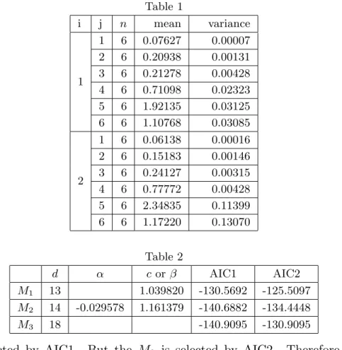
• 検索結果がありません。

Junji Moriya There is a variety of examination methods in the examination of the durability, destruction toughness value, of dental luting cement used in the field of the odontology department.

N/A
N/A
Protected

Academic year: 2021

シェア "Junji Moriya There is a variety of examination methods in the examination of the durability, destruction toughness value, of dental luting cement used in the field of the odontology department."

Copied!
4
0
0

読み込み中.... (全文を見る)

全文

(1)

不等分散をもつ関数関係モデルの選択

Selection for functional relationship models with different variances

数学専攻 守屋 順之

Junji Moriya There is a variety of examination methods in the examination of the durability, destruction toughness value, of dental luting cement used in the field of the odontology department.

Moreover, there are various materials in making cement. We want to adopt a low cost and short time method. It is necessary to examine the equality between the methods for them.

In this paper, we propose the study of the equality between two methods. We examine cements of different m materials by two methods, and obtain n samples for the cement of each material. Let a sample be x ijk , where i = 1, 2, j = 1, · · · , m and k = 1, · · · , n are methods, materials and sample numbers respectively. Suppose that x ij1 , · · · , x ijn are independently and identically distrubuted, i.i.d., according to Nij , σ j 2 ) and V ar(x 1jk ) = V ar(x 2jk

0

) = σ 2 j , k 6= k 0 . The above-mentioned can be shown like the table below.

i j sample mean variance

1 x

111

· · · x

11n

µ

11

σ

21

1 .. . .. . .. . .. . .. .

m x

1m1

· · · x

1mn

µ

1m

σ

m2

1 x

211

· · · x

21n

µ

21

σ

21

2 .. . .. . .. . .. . .. .

m x

2m1

· · · x

2mn

µ

2m

σ

m2

Let us assume that the equality expresses a linear structure between averages, and we consider the following three models.

M 1 : µ 2j = 1j , c 6= 0 (j = 1, · · · , m) M 2 : µ 2j = βµ 1j + α , β 6= 0 (j = 1, · · · , m) M 3 : otherwise

where c, α and β are unknown. It is assumed that if it is the model M 1 or M 2 , there is a functional relationship between two methods. We apply the Akaike information criterion, AIC, to evaluate these models. The AIC was proposed as the evaluation criterion of the model by Akaike (1973) and he derives the following formula.

AIC = −2(log-likelihood) + 2d, (1)

where d is the number of independent parameters. The estimators of parameters of the

log-likelihood are maximum likelihood estimators, MLEs. Let d 1 , d 2 and d 3 be d for the

(2)

M 1 , M 2 and M 3 .

d1 = 2m + 1 d2 = 2m + 2 d3 = 3m

Because x ijk i.i.d.Nij , σ j 2 ), the log-likelihood function is l =

X m

j=1

"

−n log 2π n log σ j 2 1 2σ j 2

X n

k=1

n

(x 1jk µ 1j ) 2 + (x 2jk µ 2j ) 2 o #

, (2)

where, µ 2j = 1j in the M 1 , and µ 2j = βµ 1j + α in the M 2 . Therefore, the bias of AIC is B AIC =

X m

j=1

·

(2nσ j 2 )E h 1

ˆ σ j 2

i +nE

h 1 ˆ σ j 2

n

(µ 1j µ ˆ 1j ) 2 + (µ 2j µ ˆ 2j ) 2 oi

−2n

¸ ,

where ˆ µ 2j for the M 1 and M 2 are respectively ˆ µ 2j = ˆ µ 1j and ˆ µ 2j = ˆ α + ˆ β µ ˆ 1j . Now, two problems are caused. The first is whether the usual AIC like (1) is applicable in this relational model of the function. The second is that we cannot obtain enough big n though the AIC uses the asymptotic bias. Therefore we improve the bias of AIC. We define

¯

x ij· = 1 n

X n

j=1

x ijk , s 2 ij = 1 n

X n

j=1

(x ijk x ¯ ij· ) 2 and t p,q = X m

j=1

µ p 1j σ q j .

¯

x ij· and s 2 ij are standardized and they are transformed respectively into

¯

x ij· = µ ij + 1

n u ij and n 1

n s 2 ij = σ 2 j + 1

n v ij . (3)

Let ˆ c, ˆ α and ˆ β be MLEs of c, α and β respectively. It is assumed that ˆ c, ˆ α and ˆ β are respectively extended as

ˆ

c = c + 1

n c 1 + 1

n c 2 + 1 n

n c 3 + O(n −2 ) (4)

ˆ

α = α + 1

n α 1 + 1

n α 2 + 1 n

n α 3 + O(n −2 ) (5) β ˆ = β + 1

n β 1 + 1

n β 2 + 1 n

n β 3 + O(n −2 ). (6) By using (3), (4), (5) and (6), we improved the bias for each models.

MODEL M 1

By partially differentiating (2) about c we derive the following equations. Then we may obtain the ˆ c from the following equation.

∂l

∂c = X m

j=1

x 1j· x ¯ 2j· )(¯ x 1j· + ˆ x 2j· )

(1 + ˆ c 2 )(s 2 1j + s 2 2j ) + (ˆ x 1j· x ¯ 2j· ) 2 = 0

(3)

Let ˆ µ 1j and ˆ σ j 2 be MLEs of µ 1j and ˆ σ j 2 for the model M 1 . They are obtained as follows.

ˆ

µ 1j = 1

1 + ˆ c 2x 1j· + ˆ x 2j· ) ˆ

σ j 2 = 1 2n

X n

k=1

n

(x 1jk µ ˆ 1j ) 2 + (x 2jk ˆ µ 1j ) 2 o The bias of AIC is improved as

B 1 = 2(2m + 1) + 1 n

½

4(m + 2) + 4(m 1) 1 + c 2

1

t 2,2 2 t 4,4

t 2 2,2

¾

+O(n

32

).

MODEL M 2

By partially differentiating (2) in α and β we derive the following equations. Then we may obtain the ˆ α and ˆ β from the following simultaneous equations.

∂l

∂α = X m

j=1

β ˆ x ¯ 1j· x ¯ 2j· + ˆ α

(1 + ˆ β 2 )(s 2 1j + s 2 2j ) + ( ˆ β x ¯ 1j· x ¯ 2j· + ˆ α) 2 = 0

∂l

∂β = X m

j=1

( ˆ β x ¯ 1j· x ¯ 2j· + ˆ α)(¯ x 1j· + ˆ β x ¯ 2j· )

(1 + ˆ β 2 )(s 2 1j + s 2 2j ) + ( ˆ β x ¯ 1j· x ¯ 2j· + ˆ α) 2 = 0

Let ˆ µ 1j and ˆ σ j 2 be MLEs of µ 1j and ˆ σ j 2 for the model M 2 . They are obtained as follows.

ˆ

µ 1j = 1 1 + ˆ β 2

³

¯

x 1j· + ˆ β x ¯ 2j· α ˆ β ˆ

´

ˆ σ j 2 = 1

2n X n

k=1

n

(x 1jk µ ˆ 1j ) 2 + (x 2jk α ˆ β ˆ µ ˆ 1j ) 2 o

The bias of AIC is improved as B 2 = 2(2m + 2) + 1

n

½

4(m + 4) + 4(m 2) 1 + β 2

t 0,2

t 0,2 t 2,2 t 2 1,2 2 R

¡ t 0,2 t 2,2 t 2 1,2 ¢ 2

¾

+O(n

32

), where

L j = t 2,2 2µ 1j t 1,2 + µ 2 1j t 0,2 and R = X m

j=1

1 σ j 4 L 2 j .

MODEL M 3

Let ˆ µ 1j , ˆ µ 2j and ˆ σ 2 j be MLEs of µ 1j , µ 2j and σ j 2 for the model M 3 respectively. They are ˆ

µ 1j = ¯ x 1j· , µ ˆ 2j = ¯ x 2j· and ˆ σ j 2 = 1

2 (s 2 1j + s 2 2j ).

The bias of AIC is improved as

B 3 = 2(3m) + 1

n 10m + O(n

32

).

(4)

These improved biases show that biases of the usual AIC is twices the number of parameters.

NUMERICAL RESULT

We give an example of data of dental luting cement by using the improved bias. The data is that cements of different 6 materials is examined by two methods. The sample sizes are all 6. Means and variances of data are shown by Table 1. Table 2 shows the result of the data by the usual AIC(AIC 1) and the AIC using the improved bias(AIC 2), where d is the number of parameters for each model.

Table 1

i j n mean variance

1

1 6 0.07627 0.00007 2 6 0.20938 0.00131 3 6 0.21278 0.00428 4 6 0.71098 0.02323 5 6 1.92135 0.03125 6 6 1.10768 0.03085

2

1 6 0.06138 0.00016 2 6 0.15183 0.00146 3 6 0.24127 0.00315 4 6 0.77772 0.00428 5 6 2.34835 0.11399 6 6 1.17220 0.13070

Table 2

d α c or β AIC1 AIC2

M

1

13 1.039820 -130.5692 -125.5097

M

2

14 -0.029578 1.161379 -140.6882 -134.4448

M

3

18 -140.9095 -130.9095

The M 3 is selected by AIC1. But the M 2 is selected by AIC2. Therefore, the equality between two methods was shown by using the improved bias.

REFERENCES

1. Akaike.H(1973). Information theory and an extension of the maximum likelihood principle In International Symposium on Information Theory, Ed.B.N.

Petrov and F. Csaki, 267-81.

2. Fujikoshi.Y. (1997). Modified AIC and Cp in multivariate linear regression.

Biometrica, 84, 707-716.

3. Kanai.F. (2007) Relationship between Different Fracture Toughness Tests Using Den-

tal Luting Cements. (in preparation)

Table 1 i j n mean variance 1 1 6 0.07627 0.00007260.209380.00131360.212780.00428 4 6 0.71098 0.02323 5 6 1.92135 0.03125 6 6 1.10768 0.03085 2 1 6 0.06138 0.00016260.151830.00146360.241270.00315 4 6 0.77772 0.00428 5 6 2.34835 0.11399 6 6 1.17220 0.13070

参照

関連したドキュメント

The inclusion of the cell shedding mechanism leads to modification of the boundary conditions employed in the model of Ward and King (199910) and it will be

In this paper, we study the generalized Keldys- Fichera boundary value problem which is a kind of new boundary conditions for a class of higher-order equations with

On the other hand, from physical arguments, it is expected that asymptotically in time the concentration approach certain values of the minimizers of the function f appearing in

Kilbas; Conditions of the existence of a classical solution of a Cauchy type problem for the diffusion equation with the Riemann-Liouville partial derivative, Differential Equations,

Answering a question of de la Harpe and Bridson in the Kourovka Notebook, we build the explicit embeddings of the additive group of rational numbers Q in a finitely generated group

Then it follows immediately from a suitable version of “Hensel’s Lemma” [cf., e.g., the argument of [4], Lemma 2.1] that S may be obtained, as the notation suggests, as the m A

In our previous paper [Ban1], we explicitly calculated the p-adic polylogarithm sheaf on the projective line minus three points, and calculated its specializa- tions to the d-th

Definition An embeddable tiled surface is a tiled surface which is actually achieved as the graph of singular leaves of some embedded orientable surface with closed braid