On Some Numerical Inversion Methods of the Laplace Transform

(1)

On Some Numerical Inversion Methods of the Laplace Transform

著者 Ueda Sei

journal or

publication title

Bulletin of the Education Faculty, Shizuoka University. Natural science series

volume 38

page range 97‑105

year 1988‑03‑23

出版者 Shizuoka University. Faculty of Education URL http://doi.org/10.14945/00008377

(2)

On Solme NuIIlerical lnversion Methods

of the Laplace Transform

Sei UBon ^,

(Received October tZ, tggZ)

SUMMARY

This ^paper^dealswith the properties of three numerical inversion'methods of the Laplace transform. The first method is by Bellman, the second and the third are'by the use of numerical integration and FFT algorithm. ^Thecomparisons of applicablity and accuracy among.the three methods are carried out by ^showing^some^numericalexamples. And the respective characteristcs of three methods are investigated. Bellman's method which needs few values in Laplace transform domain is suitable for stational functions. ^Themethods by numerical integration 'and

FF T algorithm which need a 'lot of values are suitable for all function types.

1. INTRODUCTION

The fundamental importance of the Laplace transform resides in its ability to lower the transcendence level of an equation. Ordinary differental equations are reduced to algebraic equations, as are also various class of integral equations involving convolutions; partial differental equations'are ^reducedto ordinaly differential equations. Then the Laplace transform technique is useful to analyze the phenomena in physical world with time variable factor.

However, it takes ^placeso frequently that the solutions in the Laplace transform domain are too compolicated to carry out the inverse transform analytically or can be obtained

only numerically. For these cases, we must use the numerical inversion technique of the Laplace transform. And the some numerical inversion methods of Laplace transform have been reported.(1)-t4)

Atthough these methods have own characteristics for CPU time, accuracy and the applicable function types, few researches on the comparison for these characteristics have been reported.

In the present paper, we investigate the each characteristics of three methods by showing some numerical examples. These three methods are representative numerical inversion techniques of the Laplace transform. ^Thefirst method is by Bellman, the second

(3)

Sei UBre

and the third method are by the use of numerical integration and FFT algorithm。

2。 NUMERiCALiNVERSiON METHODS OFttHE LAPLACE TRANSFORM

Define a Laplace transform pair by

F Ч κ)=ルけ )ο一

'α:,Fけ )=嘉 IrFЧ ^κ^)〆^み^dκ

where Br denotes the Bromwich path of integration.

2. l Numerical inverslon method by Benman

The numerical inversion formula used is as f01lows(1):

F*(κ /β)=f卜し )C―^Zン^βα ι=β

逃

勧 κ ノ lF(一

βlog χJ)

given by

WJ・==;fL戸 _{巧雨可デ蟄丼}

「受轟1丁覇理葛丁ακ

Fけ)〒 fr/1F*(σ ^十^:ω^)θ^如^'dω

wlere Rc[F*(σ+̀ω)]=Re[F*(σ^二

̀ω )], Then Eq。 (5)bOcOmes

F(;)=千

ル Чσ

^tt Jω ^)Cわ^'α

ω

WheFe _βtiS a parameter to datermine the time scalQ幼_(ノ=1,N)are zerQs Of the shifted OFdCr Legender polynomials PN(1二 2κ),and勧 (プ=1,N)‐are a sOt of weitthts which arc

(2)

0)

In Eq.(3), Pn( )are ^theLegendre polynomials of order I[and P;( 1-2x) is used for

dPr(L-2n)/d(I-2r). ;

2. 2 Numerical inversion method by use of numerical integration along the lines parallel to the

irnaginary axis _i

In Eq. (1), we substitute rc f.ar

tc:o*iu ;σ >0 ₍₄₎

and it follows that ^d,rc--id,u. ^Then^the^Laplacetransform can be converted into the integral form along the lines parallel to the imaginary axis. ^Andit should be considered that all residual point of F*( o*ia) ^mustlie to the ^left-handside of the path of integration.

(助

I興[F*(σ+Jω )]■―Im[F*(lσtt J ω)].

(0

(4)

On Some Numerical Inversion Methods of the ^LaplaceTransform 99

By carring out the integration in Eq。 (6),wc can Obtain F(:)in the time space.

2.3 Numerical inverslon methol′ by use of FFT algorithm

ln Eq。 (5),the integral form is the Fourier transform.For the evaluation ofthe FOurier integrals with the digital computer, the so‐called discrete Fourier transforIIn is used. It results froln the continuous formula if only a finite tilne interval T is consideredi thiS iS divided into Ar equidistant segments and the integration is performed by using the Euler formula13)

F(ん Zτ)=2雪

■二

^F*(σ^tt jπ

∠ ω

^)θ

″ π π ん

/N

(λ=0,1,…^…N‑1)

Hs /, ^F^{*(i^)}e"'d,u ^(s)

where Ar:T/N,Au:2 x/7. ^TodecreasetheCPUtime, we usethe algorithmof theFFT to Eq. ^(7).

2,4.Numerical inversion method by use of integral path along the imaginary axis In Eq. ^(e),the integral path is converted along the imaginary axis by ^puttinga : _0._If

the r : 0 is the residual point of F *( i r), this case is occured frequently in ^physical

phenomena, and another residual points lie to the left.hand side of the imaginary axis, then the Bromwich integral path can be converted into the path Cu * ^Co* Cr shown in Fig. 1'n). If the integration on Co can be obtained analytically, carriying out the integrations along the imaginary axis Cu * C' by numerical integration or by use of FFT algorithm, we can obtain

F(t) ⁱⁿ^the^time^space^as^follows.

１

＋万

ｄω ω θ

ｒＦ

︲ｉｍん

¨ ７１

Ｆ

CECu■CO・Ct

The contours of integration for the integral in (8)

/1n κ

Fig。 1.

(5)

Sei Unln

3.丁RIAL FUNCT10NS ' ^‐

To compare above numerical inversion methods,we intrOduce 7 kind of functibns as follows. Thesё finctions can be grouped ihtoithree tyles whiё h are the statinary,pulse and vibration typё。 1

(1)Statianary Type

(a)

Fけ )=∬(3) F*(κ

)=+

°

Fけ )二d■ (手 ⁾

F Чκ)=市

[

[″ 0→ ―″け‑1)]+″_(:‑1)

f― ^たθ

″

]十^÷ ^θ

κ

(ι ^T‐:)]‐_・ ^‐[ 1‐十 θ^'十卜

,in(?ι T̲1)

]+θ ^矛

(κ+1)2+4

l101

(C)

Fけ)=2'

F*(κ)=手

(2) Pulse type

(d)

Ir, ^r)-H

I ^t- ^e-i/z

″(〕一

:)llll

l121

F(〕 )=″ →―∬(ι‑2)

FЧa=ギ

°

F'I)=dn(子 _)[″

け

^)一

∬ け

=2)]

F*(κ)=ザ ^1̲θ

‑2″ Ａ^うツ

い

κ^2+(,2

(3)vibration type

(f)

F(:)=sin(π ι)

FЧκ)=滞

に⁾

Fけ )=cos(π ι)

F')=瀞

ハツんい

ハツ白い

(6)

On Some Numerical Inversiou Methods of the Laplace Transform

4. NUMERICAL RESULTS AND DISCUSSION

In the ^irseof Bellman's method, a too large N ^makesthe sinrultaneous equation

ill-conditiond. Then we adopedN: S, time scaleF : _1.0,L.L,I.2,1.3, L.4. ^Forthe^caseof

using FFT algorithm, Krings(3) shows that it is best to work with 101?( o<3/ _T_for_vibration

problems. Thenweuse T: ^100,o:5/T _andN:2t0.And numerical integration is carried out by use of same point values of FFT.

To examine the properties of three inve,rsion methods, inverted values are plotted in Fig. 2-Fig. 9. ^Inverted^values^ofEq. (9) are caluculated by Bellman, Rumerical integral and FFT method are shown in Fig" 2. Bellman's method can reproduce.F( l) exactly. Numerical integral method appears ZYo error. FFT method appears 207o error. This 20% error is caused by unsuitableness of parameters.

2

F(￨)

￨

Fig。 2. Inverted

23 t

values of function ^(u)

F綺卜sh続1/21H付卜Hけ,11+H‖ ―^￨)

0・・・・ °

・・ °・ ● ●00● ●0●● ● ● ● ● ● ● ●0● ● ● ●0●

A Bellman _・ Numerical lntegrol o FF丁

0

FII}=HII)

o o o o o c o o,0 o o o € o 0 o ^o

ffi

Numericol Integrr

a Bellmon . FFTNumericol Integrol o trtrT

23 t

Inverted values of function ^(b)

―￨

2

4 0

F{￨〕

0

―￨

0 4

Fig。 3.

(7)

I02 ^Sei^UBna

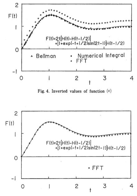
Fig. 3. and Fig. 4 are plotted the inverted ^valuesof Eqs.ftO), 0t) and show the same tendency of ^Fig.^2.

2

F(￨}

￨

o oo o o

o ooo

""rrF\--oo^

"r{

-\\ooooooooooooo6oooooo o/'

"/

.-f oA s111=4t[Hn)-Hn- | /zt]

f ^*[t*expt-^t+l/?IJinlzt-lll1nl lzl

" Bellmon ' Numericol Iniegrol

。 FF丁 0

―￨

0 4

t

Fig.4. Inverted values of function ^(c)

2

F付)舌

1蝿I缶

聟綺

^%rJn腱

卜

^1lH軒J/2)

。FF丁

0 1 2 1 3 1 4

Fig.5.Inverted values of function(C)by FFT(σ ==18/T) FII)

0

―￨

(8)

Orl Sone Numerical Inversion Methods of the Laplace Transform

Fig:5'is plotted the inverted values of Eqo a〕 by use of FFT algorithm with parameter chOsen to minimize the erroF.In this case,the parameters are σ=18/T,T=100,Ⅳ =210.

And inv∝ted values by uselof the integral path alo五g the imagillary axis are corresponded to the values of Fig。 5。

I Fig.6 shOws the inverted values in Eq:l121 by three methOds. For the case by Bellman's method,theierFoF inCreses at t==1. By numericaliintegral method and FFT method,Gibbs phenomena occured at ι=2.

2

F(￨}

￨

2

F{￨)

￨

0

―_￨

F(￨}=H{￨}―H(￨=2}

昌_ム

ム ^￨

―

￨

一 '

― △

d ttlegr。￨

JⅢ

l e rlc

I Nu撃

n . FFl

)lim o

A Bc

0 4

0

―￨

Fig。6. Inverted values of functiOn(d)

F ^(t)=s inlnt / ^Zt[H^tt^t-H^(t^-2^]l

ハ A △

Bellmon ^.Numericol lntegrol

. _FFT

t

Fis.7. Inverted values of function (")

3 4 0 2

(9)

Sei UEDA

Fig. ? shows the inverted values in Eq. ^(tt16t three methods. Error increses at t:

1.5 by Bellman's method. By the case of FFT and numerical integration are corresponded to each other cornpletely. Then the merks o of FFT values are piled up the ones of numerical integral values.

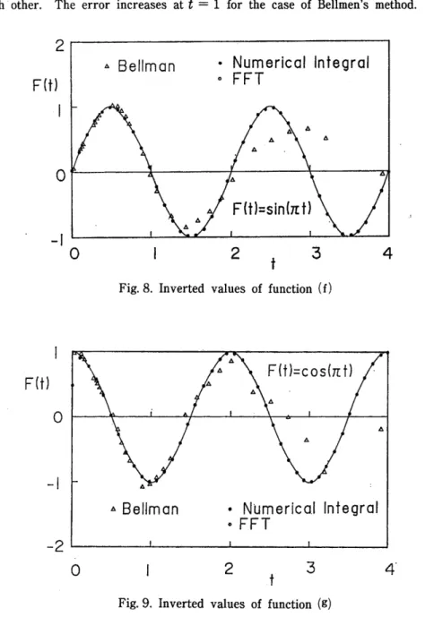
Fig.8 and Fig.9 show the values of Eqs. 04 and 05). They show the same tendency each other. The error ^increasesat t - ^{1 for}^the^case^of^Bellmen's^method.

2

F(￨}

￨

1 2

ォ 3

Fig.8. Inverted values of function(f)

F(￨)

￨

Fig。 9。

23 t

Inverted values of function ^(g)

o Bellmon . Numoricol Integrol

. _FFT

F{￨)=sinlπ l)

F(￨)〓cos{πl}

" ^Bellmon . Numericol lntegrol

. _FFT

(10)

On Some Numerical lnversion Methods of the ^LaplaceTransform ¹⁰⁵

5. CONCLUSIONS

Bellman's method can satisfactorily reproduce for the stationary functions. It is the merit of this ^methodthat only a few values are sufficient for the inverting ^process.

Then this method is useful to the problems that require long CPU time to calculate the values in the Laplace transform domain.

Numerical integral method can reproduce all function types, since a few parameters are

required. But it takes the ^longestCPU time to caluculate the inverting ^process.

FFT method can reproduce all function types, too. ^Butit requires the choice of suitable parameters. If suitable parameter are obtained, this method can carry out the inversion process in the shrtest time. In this paper, suitable parmeter a is 18/T for statinary functions and 5/T for pulse and vibrational functions.

Numerical inversion method by use of integral path along the imaginary axis is useful to reduce the CPU time to caluculate the values in Laplace transform domain.

ACKNOWLEGMENTS

The auther is grateful to Prof. T. ^{Hata and}Prof. N. Sumi, Shizuoka University, for their invaluabie directions.

REFERENGES

R. E. Bellman, R. E. Kalaba and J. Lokett, Numerical Inversion of the Laplace Transform, Elsevier Publishing Co, London, (1966).

M. K. Miller and W. T. Guy, 'Numerical Inversion of the Laplace Transform by Use of Jacobi Polynomials,' J. ^Numer.Anal. 3-4, 624-635 ^(1966).

W. Krings and H. Waller, 'Contribution _{to the}Numerical Treatment of Partal Differential Equations with the Laplace Transformation-An Application of the Algorithm of the Fast Fourier Transformation,' Int. J. Numer. Methods Eng. 14, 1183-1196 ^(1979).

J. C. ^{Pect and}J. Miklowitz, 'Shadow-zone Response in the Diffraction of a ^Plane

Compressional Pulse by a Circular Cavity'Int..J. Solids & Structures, S-5, 437-454 (1e6e).

(4)

3.

4。

2.

On Some Numerical Inversion Methods of the Laplace Transform

ル Чσ

ω

■二

∠ ω

″ π π ん

)=+

°

け

∬ け

聟 綺

卜

JⅢ

聟綺