When it is not sinθ, a new type of bifurcation phenomenon is found due to the discontinuity of the projection operator to the center subspace

Hayato Chiba

Institute of Mathematics for Industry, Kyushu University, Fukuoka 819-0395, Japan Isao Nishikawa

Institute of Industrial Science, University of Tokyo, Tokyo 153-8505, Japan (Dated: September 16, 2011)

A bifurcation theory for a system of globally coupled phase oscillators is developed based on the theory of rigged Hilbert spaces. It is shown that there exists a finite-dimensional center manifold on a space of generalized functions. The dynamics on the manifold is derived for any coupling functions. When the coupling function is sinθ, a bifurcation diagram conjectured by Kuramoto is rigorously obtained. When it is not sinθ, a new type of bifurcation phenomenon is found due to the discontinuity of the projection operator to the center subspace.

The dynamics of systems of large populations of cou- pled oscillators have been of great interest because collec- tive synchronization phenomena are observed in a variety of areas. The stability of (de)synchronous states and bi- furcations from them are the main issues to understand the behavior of systems. Since usual stability and bifur- cation theory in dynamical systems are not applicable to such systems when the dimensions of systems are too large, much work has been done to understand the dynamics.

However, except for special simple cases, to investigate bi- furcations is a quite difficult problem and much remains unclear. In this paper, a correct bifurcation theory for such systems is proposed by means of the theory of gen- eralized functions, which is applicable to large classes of coupled phase oscillators including the Kuramoto model.

To use a space of generalized functions is suitable to study the behavior of statistical quantities such as the order pa- rameter. This will be demonstrated for two cases. For the Kuramoto model, a well known Kuramoto’s bifurcation diagram will be rigorously obtained. For a certain system including the second harmonic in the coupling function, a new type of bifurcation phenomenon will be found.

INTRODUCTION

Collective synchronization phenomena are observed in a variety of areas, such as chemical reactions, engineering cir- cuits, and biological populations [1]. In order to investigate such phenomena, a system of globally coupled phase oscilla- tors of the following form is often used:

dθk

dt =ωk+K N

N j=1

f(θj−θk), k=1,· · ·,N, (1) where θk(t) denotes the phase of a k-th oscillator, ωk ∈ R denotes its natural frequency drawn from some distribution function g(ω), K > 0 is the coupling strength, and f(θ) = _∞

n=−∞fne^inθ is a 2π-periodic function (i = √

−1). When f(θ)=sinθ, it is referred to as the Kuramoto model [2]. In this case, it is numerically observed that ifKis sufficiently large, some or all of the oscillators tend to rotate at the same velocity

K

r

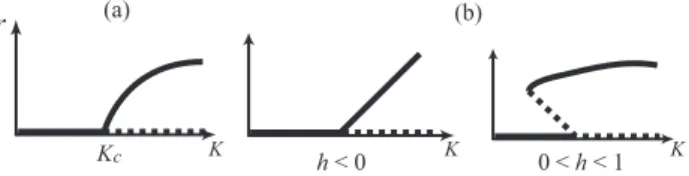
c ^K h < 0 ^K 0 < h < 1 K

(a) (b)

FIG. 1. Bifurcation diagrams of the order parameter for (a) f(θ) = sinθand (b) f(θ) = sinθ+hsin 2θ. The solid lines denote stable solutions, and the dotted lines denote unstable solutions.

on average, which is referred to assynchronization[1, 3]. In order to evaluate whether synchronization occurs, Kuramoto introduced the order parameterr(t)e^iψ(t), which is given by

r(t)e^iψ(t):= 1 N

N j=1

e^iθj(t). (2) When a synchronous state is formed, r(t) takes a positive value. Indeed, based on some formal calculations, Kuramoto assumed a bifurcation diagram ofr(t): Suppose N → ∞. If g(ω) is an even and unimodal function such thatg(0) 0, then the bifurcation diagram of r(t) is as in Fig.1(a). In other words, if the coupling strengthKis smaller thanKc := 2/(πg(0)), then r(t) ≡ 0 is asymptotically stable. If K ex- ceedsKc, then a stable synchronous state emerges. Near the transition pointKc,ris of orderO((K−Kc)^1/2). See [3] for Kuramoto’s discussion.

In the last two decades, several studies have been performed in an attempt to confirm Kuramoto’s assumption. Daido [4]

calculated steady states of Eq. (1) for anyfusing an argument similar to Kuramoto’s. Although he obtained various bifurca- tion diagrams, the stability of solutions was not demonstrated.

In order to investigate the stability of steady states, Strogatz and Mirollo and coworker [5–8] performed a linearized anal- ysis. The linear operatorT1, which is obtained by linearizing the Kuramoto model, has a continuous spectrum on the imag- inary axis. Nevertheless, they found that the steady states can be asymptotically stable because of the existence of resonance poles on the left half plane [8]. Since the results of Strogatz and Mirollo and coworker are based on the linearized anal- ysis, the effects of nonlinear terms are neglected. However, investigating nonlinear bifurcations is more difficult because

T1has a continuous spectrum on the imaginary axis, that is, a center manifold in the usual sense is of infinite dimension. In order to avoid this difficulty, Crawford and Davies [9] added noise of strengthD>0 to the Kuramoto model. The contin- uous spectrum then moves to the left side byD, and thus the usual center manifold reduction is applicable. However, their method is not valid whenD=0. An eigenfunction ofT₁as- sociated with a center subspace diverges asD → 0 because an eigenvalue on the imaginary axis is embedded in the con- tinuous spectrum asD→0. Recently, Ott and Antonsen [10]

found a special solution of the Kuramoto model, which allows the dimension of the system to be reduced. Their method is applicable only forf(θ)=sinθbecause their method relies on a certain symmetry of the system [11]. Furthermore, the re- duced system is still of infinite dimension, except for the case in which g(ω) is a rational function. Pikovsky and Rosen- blum [12] proposed the reduction of the system based on the construction of constants of motion. Their method also relies on a special form of the system. Thus, a unified bifurcation theory for globally coupled phase oscillators is required.

In the present paper, a correct center manifold reduction is proposed by means of the theory of generalized func- tions, which is applicable for any coupling function f. It is shown that there exists a finite-dimensional center mani- fold on a space of generalized functions, despite the fact that the continuous spectrum lies on the imaginary axis. This will be demonstrated for two cases, (I) f(θ) = sinθand (II) f(θ) =sinθ+hsin 2θ,h ∈ R, and two distribution functions g(ω), (a) a Gaussian distribution and (b) a rational function (e.g., Lorentzian distribution g(ω) = 1/(π(1+ω²))). For (I), we rigorously prove Kuramoto’s conjecture; that is, it is shown for the continuous limit that when 0 < K < Kc, the de-synchronous state r ≡ 0 is locally asymptotically stable, and whenKc<K, a stable synchronous stater>0 bifurcates from the trivial solution with the orderO((K−Kc)^1/2). For (II), a different bifurcation diagram will be obtained, as was predicted by Daido [4]. The different bifurcation structure is shown to be caused by the discontinuity of the projection to the generalized center subspace. All omitted proofs are given in [13].

THE CONTINUOUS MODEL

Let us derive the continuous model (the continuum limit) of Eq.(1) to describe the situationN → ∞. By introducing the Daido’s order parameter [4]

ηˆk(t) := 1 N

N j=1

e^ikθj(t),

Eq.(1) is rewritten as dθk

dt =ωk+K ∞ l=−∞

flηˆl(t)e^−ilθk.

This implies that the flow ofθkis generated by the vector field ˆ

v=ωk+K ∞ l=−∞

flηˆl(t)e^−ilθk.

Hence, we define the continuous model of Eq.(1) as the equa- tion of continuity







∂ρt

∂t + ∂

∂θ(ρtv)=0, v:=ω+K

∞ l=−∞

flηl(t)e^−ilθ, (3) whereηlis defined to be

ηl(t)=

R

_2π

0

e^ilθρt(θ, ω)g(ω)dθdω,

g(ω) is a given probability density function for natural fre- quencies, and the unknown functionρt =ρt(θ, ω) is a proba- bility measure on [0,2π) parameterized byt, ω∈R. In partic- ular,η1is a continuous version of Kuramoto’s order parame- ter. Roughly speaking,ρt(θ, ω) denotes a probability that an oscillator having a natural frequencyωis placed at a position θ.

SettingZj(t, ω) :=_2π

0 e^{i jθ}ρt(θ, ω)dθyields dZj

dt =i jωZj+i jK fjηj+i jK

lj

flηlZj−l. (4) The trivial solutionZj≡0 (j=±1,±2,· · ·) corresponds to the uniform distributionρt≡1/2πon a circle, which impliesr≡ 0 (de-synchronous state). To investigate the stability of this state, we consider the linearized system. LetL²(R,g(ω)dω) be the weighted Lebesgue space with the inner product

(ψ, φ)=

R

ψ(ω)φ(ω)g(ω)dω.

PutP0(ω)≡1. Then, the order parameters are written as ηj(t)=

R

Zj(t, ω)g(ω)dω=(Zj,P₀)=(P₀,Zj), (5) and the linearized system of Eq.(4) is given by

dZj

dt =TjZj:=i jωZj+i jK fj(P0,Zj). (6) Let us consider the spectra of linear operatorsTj. The spec- trum ofTjconsists of the continuous spectrum and eigenval- ues. The continuous spectrum is the whole imaginary axis.

EigenvaluesλofTjare given as roots of the equation

R

1

λ−i jωg(ω)dω= 1

i jK fj. (7) Indeed, the equation (λ−Tj)v=0 provides

v+i jK fj(P0,v)(λ−i jω)⁻¹P0=0.

Taking the inner product with P0, we obtain Eq.(7). It is known that there exists a positive constant Kc^(j) such that if Kc^(j) < K,Tj has eigenvalues on the right half plane, so that the j-th Fourier component of the de-synchronous state is un- stable, while if 0<K <Kc^(j),Tj has no eigenvalues. In par- ticular, wheng(ω) is even and unimodal, there exists a unique eigenvalueλ = λ0(K) on the right half plane for Kc^(j) < K.

As K decreases, λ0(K) moves to the left, and at K = Kc^(j), λ0(K) is absorbed into the continuous spectrum on the imagi- nary axis. In this manner, the eigenvalue suddenly disappears atK = Kc^(j). For example, if f is an odd function and ifgis even and unimodal, thenKc^(j)is given by

Kc^(j)=− Im(fj)

π|fj|²g(0). (8) In the present paper, for simplicity, we assume thatKc⁽¹⁾is the least number amongK⁽c^j);Kc :=infjKc^(j) =Kc⁽¹⁾. This means that the first Fourier component of the coupling function f is the most dominant term (for f(θ)=sinθ+hsin 2θ, which is true if and only if h < 1). When 0 < K < Kc, Tj has no eigenvalues and the spectrum consists only of the continuous spectrum on the imaginary axis for any j. Thus the dynamics of the linearized systemdZj/dt=TjZjis quite nontrivial. It is well known for a finite dimensional system that the trivial so- lution is neutrally stable if the spectrum lies on the imaginary axis. For infinite dimensional systems, this is not true. Indeed, numerical simulation [8, 14] suggests that the order parame- ter decays exponentially to zero when 0<K <Kc. Strogatz and coworkers [8] found that such an exponential decay of the order parameter is induced by a resonance pole, and it is rig- orously proved by Chiba [13]. In [13], the spectral theory on rigged Hilbert spaces is developed to reveal the dynamics of the linearized system.

A RIGGED HILBERT SPACE

A rigged Hilbert space consists of three spaces X ⊂ L²(R,g(ω)dω) ⊂ X: a space X of test functions, a Hilbert space L²(R,g(ω)dω), and the dual space X of X (a space of continuous anti-linear functionals on X, each element of which is referred to as a generalized function). We use Dirac’s notation, where for µ ∈ X andφ ∈ X, µ(φ) is denoted by φ|µ . For a ∈ C, we have aφ|µ = aφ|µ = φ|aµ . A usual function can be regarded as a generalized function using an integral kernel. To be precise, the canonical inclu- sion i : L²(R,g(ω)dω) → X is defined as follows. For ψ∈L²(R,g(ω)dω), we denotei(ψ) by|ψ , which is defined to be

i(ψ)(φ)=φ|ψ :=(φ, ψ)=

R

φ(ω)ψ(ω)g(ω)dω. (9) By the canonical inclusion, Eq. (4) is rewritten as an evolution equation on the dual spaceXas

d

dt|Zj =T^×_j|Zj +i jK

lj

flP₀|Zl · |Zj−l , (10)

whereT^×_j is a dual operator ofTjdefined throughφ|T^×_jµ = T^∗_jφ|µ forµ ∈ Xandφ ∈ X, and T^∗_j is the adjoint opera- tor ofTj. In particular, for anyψ ∈ L²(R,g(ω)dω), we have φ|T^×_jψ =T^∗jφ|ψ =(T^∗_jφ, ψ)=(φ,Tjψ). ThusT^×_j gives an extension ofTjto the dual space.

Here, the strategy for the bifurcation theory of globally cou- pled phase oscillators is to use the space of generalized func- tionsXrather than a space of usual functions. The reason for this is explained intuitively as follows. If we use the space L²(R,g(ω)dω) to investigate the dynamics, then the behavior ofρt itself will be obtained. However, it is neutrally stable because of the conservation law_2π

0 ρt(θ, ω)dθ=1. What we would like to know is the dynamics of the moments ofρt, in particular, the order parameter. This suggests that we should use a different topology for the stability ofρt. (Note that the definition of stability depends on definition of the topology.) For the purpose of the present study,ρtis said to be convergent to ˆρast→ ∞if and only if

R

_2π

0

φ(ω)e^{i jθ}g(ω)dρt(θ, ω)

→

R

_2π

0

φ(ω)e^{i jθ}g(ω)dρ(θ, ω)ˆ

for any j ∈ Zandφ ∈ X. This implies that for the Fourier coefficients, a functionZj(t, ω)∈L²(R,g(ω)dω) is said to be convergent to ˆZj(ω) ast→ ∞if and only if

R

φ(ω)Zj(t, ω)g(ω)dω→

R

φ(ω) ˆZj(ω)g(ω)dω,

for anyφ ∈X. In other words,Zj(t, ω) converges to ˆZj(ω) if and only ifφ|Zj → φ|Zˆj for anyφ∈Xif we regardZjas a generalized function. The topology induced by this conver- gence is referred to as the weak topology. By the completion ofL²(R,g(ω)dω) with respect to the weak topology, we ob- tain a space of generalized functionsX. On the spaceX, a functionZ₁(t, ω) converges as t → ∞if and only if φ|Z₁ converges for anyφ∈X. Since the order parameter is written asη1(t)=P0|Z1 , this topology is suitable for the purpose of the present study. Although a solution of the linearized sys- temdZj/dt=TjZjis neutrally stable inL²(R,g(ω)dω)-sense because of the continuous spectrum on the imaginary axis, we will show that it can decay to zero exponentially if we use the weak topology. More generally, a rigged Hilbert space provides strong tools for studies of dynamics of moments of measures or probability density functions. A suitable choice of the spaceXdepends on a problem, which will be explained in the next section.

A rigged Hilbert space was introduced by Gelfand [15] to generalize the theory of Schwartz distributions. See [16] for a review of Gelfand’s work and its application to quantum me- chanics.

A SPECTRAL THEORY ON RIGGED HILBERT SPACES We give a summary of the spectral theory on rigged Hilbert spaces developed in [13]. In what follows, put f1=1/(2i) for simplicity (that is, f(θ)=sinθ+(higher harmonics)) and we consider the operator

T1φ=iωφ+K

2(P0, φ)P0.

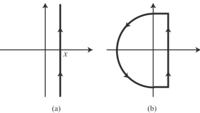
Lete^T1tφbe the solution of the linearized systemdZ1/dt= T1Z1with the initial conditionφ(ω). The linear operatore^T1tis called the semigroup (semiflow) generated byT₁. It is known that the semigroupe^T1tis given by the Laplace inversion for- mula

e^T1t= lim

y→∞

1 2πi

x+iy x−iy

e^λt(λ−T₁)⁻¹dλ, (11) for t > 0, where x > 0 is chosen so that the contour is to the right of the spectrum ofT1(see Fig.3 (a)). The operator (λ−T1)⁻¹ is called the resolvent in functional analysis (in engineering, it is called the Laplace transform). The resolvent is a continuous operator onL²(R,g(ω)dω) whenλdoes not lie on the spectrum ofT₁. SinceT₁has the continuous spectrum on the imaginary axis, the inner product (φ,(λ−T₁)⁻¹ψ) for ψ, φ ∈ L²(R,g(ω)dω) diverges whenλ ∈ iR. However, it is possible that (φ,(λ−T1)⁻¹ψ) exists on the imaginary axis and has an analytic continuation from the right half plane to the left half plane ifψandφsatisfy suitable conditions. To see this idea, it is sufficient to consider the multiplication operator iMφ:=iωφ; that is,K=0 forT1. The resolvent is given by

(φ,(λ−iM)⁻¹ψ)=

R

1

λ−iωψ(ω)φ(ω)g(ω)dω, for anyψ, φ ∈ L²(R,g(ω)dω). In general, the integral in the right hand side diverges as Re(λ) → 0 because of the fac- tor 1/(λ−iω). However, ifψandφare holomorphic on the real axis and the upper half plane, the integral converges as Re(λ)→ +0 and has an analytic continuation from the right half plane to the left half plane, which is given by

R

1

λ−iωψ(ω)φ(ω)g(ω)dω

+2πψ(−iλ)φ(−iλ)g(−iλ), Re(λ)<0.

LetXbe a vector space consisting of some class of holomor- phic functions defined near the upper half plane. The above calculation implies that (φ,(λ−iM)⁻¹ψ) is an entire func- tion when ψ, φ ∈ X. The second term of the above quan- tity is not written as an inner product of two functions. This suggests that the analytic continuation of the resolvent is no longer included inL²(R,g(ω)dω) . Since the complex num- ber (φ,(λ−iM)⁻¹ψ) exists for each φ ∈ X, we can regard (λ−iM)⁻¹ψas a functional onX; that is, an element of the dual spaceX. To be precise, define thegeneralized resolvent

A(λ) ofiMto be φ|A(λ)ψ

=



(φ,(λ−iM)⁻¹ψ) (Re(λ)>0), (φ,(λ−iM)⁻¹ψ)

+2πψ(−iλ)φ(−iλ)g(−iλ) (Re(λ)<0).

Since the mappingφ → φ|A(λ)ψ is linear, |A(λ)ψ is an element ofX. Since|A(λ)ψ is determined for eachψ∈ X, A(λ) is a linear operator fromX intoXand is analytic with respect toλ∈C. By the definition,A(λ)ψ=(λ−iM)⁻¹ψwhen Re(λ)>0. Now we have shown that the resolvent (λ−iM)⁻¹ as an operator on L²(R,g(ω)dω) diverges on the imaginary axis, however, if we regard it as an operator fromXintoX, it has an analytic continuation, which is denoted byA(λ), from the right half plane to the left half plane.

Similarly, we can prove that the resolvent (λ−T₁)⁻¹of the operatorT₁ does not exist as an operator on L²(R,g(ω)dω) whenλ∈ iR. If we regard it as an operator fromXintoX, however, it has a meromorphic continuationRλfrom the right half plane to the left half plane. PutPφ = ^K₂(P₀, φ). Then, T₁ =iM+P. The resolvent ofT₁is rewritten as

(λ−T1)⁻¹=(λ−iM)⁻¹◦(id− P(λ−iM)⁻¹)⁻¹, whereidis the identity mapping. Hence, the analytic contin- uation of (λ−T1)⁻¹in the generalized sense is given by

R_λ:=A(λ)◦(id− P^×A(λ))⁻¹, which is a linear operator fromXintoX.

The generalized resolventR_λ is a meromorphic function with respect toλ. A pole of the generalized resolvent is called ageneralized eigenvalue. A pointλis a generalized eigen- value if and only if the operatorid− P^×A(λ) is not injective onX. ForT1, generalized eigenvalues are given as roots of the equation

R

1

λ−iωg(ω)dω= 2

K, (Re(λ)>0), (12)

R

1

λ−iωg(ω)dω+2πg(−iλ)= 2

K,(Re(λ)<0). (13) In particular, a root of Eq.(13) is called theresonance pole.

Note that Eq.(12) is the same as Eq.(7) (forj=1,f1=1/(2i)).

Thus generalized eigenvalues on the right half plane are eigen- values ofT1in the usual sense. Recall that Eq.(12) has a root if and only ifK > Kc. In particular, wheng(ω) is even and unimodal, there exists a unique eigenvalueλ=λ0(K) on the right half plane forK >Kc. AsK → Kc+0, the eigenvalue λ0(K) is absorbed into the continuous spectrum on the imagi- nary axis and disappears. However, it is easy to show that even for 0<K<Kc,λ0(K) remains to exist as a root of Eq.(13) be- cause the left hand side of Eq.(13) is an analytic continuation of that of Eq.(12). This means that althoughλ0(K) disappears from the original complex plane atK = Kc, it still exists for 0 < K < Kcas a resonance pole on the Riemann surface of the generalized resolventR_λ(see Fig.2). We will show that resonance poles induce an exponential decay of a solution.

FIG. 2. The motion of the generalized eigenvalue asK decreases.

WhenK > Kc, it exists on the right half plane as an eigenvalue of T1. AtK = Kc, it is absorbed into the continuous spectrum and disappears from the complex plane. WhenK < Kc, it goes to the second Riemann sheet of the generalized resolvent and turns into a resonance pole, which is no longer an eigenvalue ofT1in the usual sense.

Letλ0, λ1, λ2,· · · be the generalized eigenvalues ofT₁and T₁^×a dual operator ofT₁. We can show that there exist gen- eralized functions µj ∈ X such that T₁^×|µj = λj|µj ; that is, generalized eigenvalues are indeed eigenvalues of the dual operator. The generalized eigenfunctionµjassociated withλj

is given by

φ|µj =









R

1

λj−iωφ(ω)g(ω)dω (Re(λj)>0),

R

1

λj−iωφ(ω)g(ω)dω

+2πφ(−iλj)g(−iλj), (Re(λj)<0).

Now that the analytic continuation R_λ of the resolvent (λ−T1)⁻¹ and its poles are obtained, the Laplace inversion formula (11) can be calculated by using the residue theorem.

Considering the spaceL²(R,g(ω)dω),T1 has the continuous spectrum on the imaginary axis, and thus we can not deform the contour of the Laplace inversion formula toward the left half plane. However, if we regard the resolvent as an operator fromXintoX, the integrand of the Laplace inversion formula has an analytic continuation to the left half plane. Indeed, the semigroup is rewritten as

(φ,e^T1tψ)= 1 2πi

x+i∞

x−i∞ e^λt(φ,(λ−T₁)⁻¹ψ)dλ,

= 1 2πi

x+i∞

x−i∞ e^λtφ| R_λψ dλ,

forψ, φ∈ X. Generalized eigenvalues are poles ofφ| R_λψ . In the following, for simplicity, we assume that allλn’s are single roots (this is true wheng(ω) is the Gaussian). By de- forming the contour as is shown in Fig.3(b), we can prove the equality

(φ,e^T1tψ)=^∞

n=0

K 2Dn

e^λntφ|µn ψ|µn , (14)

where the constantDnis defined by Dn= lim

λ→λn

1 λ−λn

1−K 2

R

g(ω)

λ−iωdω−πKg(−iλ)

,

x

(a) (b)

FIG. 3. The contour for the Laplace inversion formula.

which arises from the residue aroundλn. Since (φ,e^T1tψ) = φ|(e^T1t)^×ψ , the above equality is also written as the equality on the dual spaceXas

(e^T1t)^×|ψ =^∞

n=0

K 2Dn

e^λntψ|µn · |µn , (15) for anyψ ∈ X. This gives the spectral decomposition of the dual operator ofe^T1tusing the generalized functions.

Recall that the spaceX consists of holomorphic functions defined near the upper half plane so that the analytic contin- uation of the resolvent exists. Further, we should chooseX so that the integral of the Laplace inversion formula along the contour shown in Fig.3(b) converges for anyψ, φ ∈ Xas the radius of the arc tends to infinity. A suitable choice ofXand the distribution of resonance poles depend ong(ω).

(a)Wheng(ω) is a Gaussian distribution, let Exp₊(β) be the set of holomorphic functions defined near the upper half plane such that|φ(z)|e^−β|z|is bounded on the real axis and the upper half plane. SetX = Exp₊ :=

β≥0Exp₊(β). We can intro- duce a suitable topology on Exp₊so that the dual space Exp₊ becomes a complete metric space, which allows the existence of a center manifold on Exp₊to be proven. Since the analytic continuation ofg(ω) is a transcendental entire function, infin- ity∞is an essential singularity, which proves that Eq.(13) has infinitely many roots that accumulate at∞.

(b)Wheng(ω) is a rational function, X := H₊is a space of bounded holomorphic functions on the real axis and the upper half plane. It is remarkable that wheng(ω) is rational, Eq.(13) is reduced to an algebraic equation, so that the number of resonance poles is finite. Therefore, the right hand side of Eq.(15) is a finite sum. This implies that the semigroup (e^T1t)^× behaves as an “exponential of a matrix”. This fact is explained by means of the rigged Hilbert space as follows: AlthoughH₊ is an infinite dimensional vector space, its inclusioni(H₊) ⊂ H₊ into the dual space becomes a finite-dimensional vector space ( i.e. the canonical inclusioniis not injective). Hence, if we regard the infinite-dimensional system (4) as the system defined on the dual space by the canonical inclusion, Eq. (10) becomes essentially a finite-dimensional system. This is why in [10, 17], the system is reduced to a finite-dimension system wheng(ω) is the (sum of the) Lorentzian distribution.

Equation (15) completely determines the dynamics of the order parameter for the linearized system. The order parame- ter of the systemdZ1/dt=T1Z1with the initial conditionψis given as

η1(t)=(P0,e^T1tψ)=P0|(e^T1t)^×ψ .

If 0<K <Kc, then all generalized eigenvaluesλnlie on the left half plane. As a result,η1(t) decays to zero exponentially as t → ∞, which proves the asymptotic stability of the de- synchronous state.

The other operatorsT₂,T₃,· · · are investigated in the same way. Due to the assumption infjKc^(j) = Kc⁽¹⁾ = Kc, all gen- eralized eigenvalues of Tj(j 1) lie on the left half plane when 0 <K ≤ Kc. Thusηj =P0|(e^Tjt)^×ψ decays to zero exponentially ast→ ∞.

CENTER MANIFOLD REDUCTION

WhenK > 0 is sufficiently small, all resonance poles lie on the left half plane. AsKincreases, they move to the right side, and whenK=Kc, there exist resonance poles (ofT1) on the imaginary axis. It is well known that a bifurcation occurs when an eigenvalue gets across the imaginary axis as a param- eter varies. Let us show that a bifurcation also occurs when a resonance pole gets across the imaginary axis.

For each j, |Zj is an element of the dual space X. Let X_j(j = ±1,±2,· · ·) be copies of X. We regard the system Eq.(10) as an evolution equation on

j0X_j. The general- ized center subspaceEcis defined as a space spanned by gen- eralized eigenfunctions associated with resonance poles on the imaginary axis, say λ0,· · ·, λM, which exist only when K = Kc. Since resonance poles ofTj(j 1) lie on the left half plane,Ec ⊂ X₁. Equation (15) suggests that the projec- tionΠctoEcis given by

Πc|ψ = M n=0

K

2Dnψ|µn · |µn . (16) Unfortunately, Πc : X ⊂ X → X is not continuous be- cause the topology on X is too weak; when|ψ → 0 inX, Πc|ψ does not tend to zero in general. When X = Exp₊ = β≥0Exp₊(β), it is proven in [13] that Πc becomes a con- tinuous operator if the domain is restricted to the subspace i(Exp₊(0)) ⊂ X. For a solution of Eq. (4), Z1,Z2,· · · are included in Exp₊(0) (if initial conditions are), although Z₋₁,Z₋₂,· · · are not. To see this, again it is sufficient to con- sider the case K = 0. In this case, Tjφ = i jωφ and the solution of the equation dZj/dt = TjZjwith the initial con- ditionφ ∈ Exp₊(0) is given byZj(t, ω) = e^{i jωt}φ(ω). When j ≥ 1, e^{i jωt} is bounded uniformly in Im(ω) ≥ 0 andt ≥ 0, so thatZj(t, ω) ∈ Exp₊(0) for anyt ≥ 0. On the other hand, when j < 0, e^{i jωt} diverges as |e^{i jωt}| ∼ O(e^|jt|·Im(ω)), so that Zj(t, ω)Exp₊(0). Hence, ifi(Zj(t))=|Zj converges to zero ast→ ∞,Πc|Zj tends to zero when j≥1, although it may not tend to zero when j < 0. In the usual center manifold

theory, the projection to a center subspace is assumed to be continuous. Because of the discontinuity ofΠc, an interesting bifurcation occurs when f(θ) sinθ. In what follows, as- sume thatgis an even and unimodal function. In this case, on the imaginary axis,T1has only one resonance poleλ0=0 at K=Kc. Hence,

Ec=· · · × {0} × {0} ×span{µ0} × {0} × {0} × · · · ⊂

j0

X_j is of one dimension, whereµ0is the generalized eigenfunction associated withλ0=0, which is given by

φ|µ0 := lim

λ→+0

R

1

λ−iωφ(ω)g(ω)dω. (17) This is also written as

|µ0 = lim

λ→+0 1 λ−iω

,

where the limit is taken with respect to the weak topology.

The complementary subspaceE^⊥_c ofEcin

j0X_jis the sta- ble subspace. Next, let us derive the dynamics on a center manifold. The derivation is performed in the same way for both (a) a Gaussian distribution and (b) rational functions.

(I)First, we consider f(θ)=sinθ. In this case, Eq. (10) is reduced to

d

dt|Z1 =T₁^×|Z1 −K

2P0|Z1 |Z2 , (18) and

d

dt|Zj =T^×_j|Zj − jK 2

P0|Z1 |Zj+1 − P0|Z1 |Zj−1

, (19) for j = 2,3,· · ·. It is remarkable that these equations of

|Z1 ,|Z2 ,· · · are independent of|Z₋₁ ,|Z₋₂ ,· · ·. Therefore, the projectionΠc continuously acts on these equations. In order to investigate a bifurcation occurred at K = Kc, set ε=K−Kc. Then, Eq. (18) is rewritten as

d

dt|Z₁ =T₁₀^×|Z₁ +ε

2P0|Z₁ |P₀ − K

2P0|Z₁ |Z₂ , (20) whereT10is defined by

T₁₀φ=iωφ+Kc

2 (P₀, φ)P₀,

andT₁₀^× is its dual operator. Note that T10 has a resonance poleλ0 = 0. In order to obtain the dynamics on the center manifold, we decompose a solution as

|Z1 = Kc

2 α|µ0 +|Y1 , (21) along the direct sumEc⊕E^⊥_c. Theαrepresents the coordinate on the center subspace, which is assumed to be sufficiently small;|α| << 1. The purpose here is to derive the dynamics ofα. Since|Y1 and|Z2 are included in the stable subspace,

they are higher order terms with respect to α; |Y1 ,|Z2 ∼ O(α²).

Due to the definitions ofµ0and the resonance pole, we ob- tainP0|µ0 =2/Kc. This provides

P0|Z1 =α(t)+P0|Y1 . (22) The projection of|P₀ is given by

Πc|P0 = Kc

2D0P0|µ0 · |µ0 = 1 D0|µ0 . Hence,|P0 is decomposed as

|P0 = 1

D0|µ0 +|Y0 , (23) where |Y0 ∈ E^⊥_c and |Y0 ∼ O(α²). Substituting Eqs.(22),(21) into Eq.(19) for j=2 yields

d

dt|Z2 =T₂^×|Z2 −K

(α+P0|Y1 )· |Z3

−(α+P₀|Y₁ )Kc

2 α|µ0 +|Y₁

. (24) We suppose thatdα/dt∼O(α², αε, ε²). Then, the above equa- tion yields

T₂^×|Z2 =−KKc

2 α²|µ0 +O(α³, α²ε, αε², ε³). (25) Lemma 1. Define the operator (T₂^×)⁻¹:X→Xto be

φ|(T₂^×)⁻¹ψ =−1 2 lim

x→+0

R

1

x−iωφ(ω)ψ(ω)g(ω)dω.

Then,

(T₂^×)(T₂^×)⁻¹|ψ =(T₂^×)⁻¹(T₂^×)|ψ =|ψ (26) for anyψ∈X.

Proof. Note thatT2φ =2iωφwhen f(θ)=sinθ. A straight- forward calculation shows that

φ|(T₂^×)(T₂^×)⁻¹ψ

=T₂^∗φ|(T₂^×)⁻¹ψ

=−1 2 lim

x→+0

R

2iω

x−iωφ(ω)ψ(ω)g(ω)dω

=

R

φ(ω)ψ(ω)g(ω)dω− lim

x→+0

R

x

x−iωφ(ω)ψ(ω)g(ω)dω

=

R

φ(ω)ψ(ω)g(ω)dω.

Thus we obtain

φ|(T₂^×)(T₂^×)⁻¹ψ =φ|ψ ,

for anyφ∈ X. The latter equalityφ|(T₂^×)⁻¹(T₂^×)ψ =φ|ψ

is proved in the same way.

Using the definition ofµ0, (T₂^×)⁻¹|µ0 is calculated as φ|(T₂^×)⁻¹µ0 = lim

x→+0

φ(T₂^×)⁻¹ 1 x−iω

=−1 2 lim

x→+0

R

1

(x−iω)²φ(ω)g(ω)dω. (27) Then, Eq.(25) provides

φ|Z2 =KKc

4 α² lim

x→+0

R

1

(x−iω)²φ(ω)g(ω)dω +O(α³, α²ε, αε², ε³), (28) which gives the expression of the center manifold to the|Z2

direction. The projection of it to the center subspace is given as

Πc|Z2 = Kc

2D0Z2|µ0 · |µ0

= Kc

2D0 xlim→+0

Z₂ 1 x−iω

· |µ0

= Kc

2D₀ lim

x→+0

1 x+iωZ2

· |µ0 .

In what follows, higher order terms with respect toαandεare denoted by h.o.t. Eq.(28) yields

xlim→+0

1 x+iωZ₂

= KKc

4 α² lim

x→+0

R

1

(x−iω)³g(ω)dω+h.o.t.

=−KKc

8 α² lim

x→+0

R

1

x−iωg(ω)dω+h.o.t.

=−KKc

8 α²·πg(0)+h.o.t.

For the last equality, we used a formula of the Poisson kernel.

Thus we obtain

Πc|Z2 =−KK_c²

16D₀α²·πg(0)· |µ0 +h.o.t. (29) Finally, the projection of Eq.(20) to the center subspace is given by

d

dtΠc|Z₁ = ΠcT₁₀^×|Z₁ +ε

2P0|Z₁ Πc|P₀ − K

2P0|Z₁ Πc|Z₂ . Recall that a resonance pole is an eigenvalue of the dual op- erator. SinceΠcis a projection to the eigenspace associated with a resonance poleλ0=0 ofT₁₀^×, we have

ΠcT₁₀^× =T₁₀^×Πc=0. (30) By using Eqs.(21),(22),(23),(29) and (30), we obtain

d dt

Kc

2 α|µ0

= ε

2(α+P0|Y1 ) 1 D0|µ0

−K

2(α+P₀|Y₁ )· −πg(0)KK_c²

16D0 α²|µ0 +h.o.t.

,

= ε

2D0α|µ0 +πg(0)K_c⁴

32D0 α|α|²|µ0 +h.o.t.,

which yields the dynamics on the center manifold as d

dtα= α

D0Kc ε+πg(0)K_c⁴ 16 |α|²

+h.o.t. (31) Sinceg(0) < 0 for the Gaussian distribution, this equation has a fixed point expressed as

α=

−16 πKc⁴g(0)

K−Kc+O(K−Kc), (32)

whenε=K−Kc>0. Note that Kuramoto’s order parameter η1(t)=(P₀,Z₁) is given as

η1(t)=P0|Z₁ =α+h.o.t. (33) Thus the dynamics of the order parameter is also given by Eq.(31). To prove that the fixed point (32) is asymptotically stable, it is sufficient to show the following.

Lemma 2. D0>0.

Proof. This is proved by using the definition ofD0

D₀=lim

λ→0

1

λ 1−Kc

2

R

g(ω)

λ−iωdω−πKcg(−iλ)

, and the fact thatg(ω) is an even and unimodal function. See

[13] for the details.

Since D₀ > 0,Kc > 0,g(0) < 0, the fixed pointα = 0 (de-synchronous state) is unstable and the fixed point Eq.(32) (synchronous state) is asymptotically stable when ε = K− Kc>0. This confirms the Kuramoto’s bifurcation diagram.

(II)Assume that f(θ)=sinθ+hsin 2θwithh ∈R. Then, Eq. (10) is reduced to

d

dt|Z1 =T₁₀^×|Z1 +ε

2P0|Z1 |P0

−K 2

P₀|Z₁ |Z₂ +hP₀|Z₂ |Z₃ −hP₀|Z₂ |Z₋₁ , (34) and

d

dt|Z2 =T₂^×|Z2

−K

P0|Z1 |Z3 +hP0|Z2 |Z4 − P0|Z1 |Z1

, (35) for j=1,2, respectively, where

T₂φ=2iωφ+Kh(P₀, φ)P₀. (36) Note that Eq.(34) includes|Z₋₁ , on whichΠcis a discontin- uous operator. Eq.(35) provides

T₂^×|Z2 =−KKc

2 α²|µ0 +h.o.t. (37) as before.

Lemma 3. Define the operator (T₂^×)⁻¹ :X→Xto be φ|(T₂^×)⁻¹ψ =−1

2 lim

x→+0

R

1

x−iωφ(ω)ψ(ω)g(ω)dω

−Kh 2

1

2−hKπg(0) lim

x→+0

R

φ(ω)g(ω) x−iω dω·

R

ψ(ω)g(ω) x−iω dω.

Then,

(T₂^×)(T₂^×)⁻¹|ψ =(T₂^×)⁻¹(T₂^×)|ψ =|ψ (38) for anyψ∈X.

This lemma is verified by a straightforward calculation as the proof of Lemma 1. This is applied to Eq.(37) to yield

φ|Z₂ =−KKc

2 α²φ|(T₂^×)⁻¹µ0 +h.o.t.

= K_c² 4 α² lim

x→+0

R

1

(x−iω)²φ(ω)g(ω)dω +1

4

K_c³hα² 2−hKcπg(0) lim

x→+0

R

φ(ω)g(ω) x−iω dω

R

g(ω) (x−iω)²dω +h.o.t.

Define the negative constantCto be C=− lim

x→+0

R

g(ω)

(x−iω)²dω=p.v.

R

g(ω)

ω dω. (39) Sinceg(ω) is assumed to be even and unimodal, Eq.(8) pro- vides

Kc=K⁽¹⁾_c = 2

πg(0). (40)

Hence, we obtain φ|Z2 =K_c²

4 α² lim

x→+0

R

1

(x−iω)²φ(ω)g(ω)dω

−Kc³Chα² 8(1−h) lim

x→+0

R

φ(ω)g(ω)

x−iω dω+h.o.t.

In particular,

P₀|Z₂ =−K_c²

4 α²C−K_c³Chα²

8(1−h)πg(0)+h.o.t.

=− K_c²C

4(1−h)α²+h.o.t. (41) Since|Z2 ∼O(α²) andΠccontinuously acts on|Z2 ,Πc|Z2

is also of order α². Similarly, we have Πc|Z₃ ∼ O(α²).

Hence,

P0|Z1 |Z2 ∼O(α³), P0|Z2 |Z3 ∼O(α³). (42) Substituting Eqs.(21),(22),(23),(30),(41) and (42) into Eq.(34), we obtain

d dt

Kc

2 α|µ0 = εα

2D0|µ0 − Kch 2

K²_cC

4(1−h)α²·Πc|Z₋₁ +h.o.t.

(43)