福岡工業大学学術機関リポジトリ

Title

Extrapolated Absorbing Boundary Condition for FDTD Analysis

Author(s)

Hiroshi MAEDA

Citation

福岡工業大学研究論集　第39巻第2号P3-P11

Issue Date

2007

URI

http://hdl.handle.net/11478/365

Right

Type

Research Paper

Textversion publisher

福岡工業大学　機関リポジトリ　

FITREPO

Extrapolated Absorbing Boundary Condition for FDTD Analysis

Xuefeng LI (Intelligent Information System Engineering)

Hiroshi MAEDA (Department of Communication and Computer Engineering)

Kazunori UCHIDA (Department of Communication and Computer Engineering)

Abstract

In this paper a novel absorbing boundary condition for the finite difference time domain (FDTD) method based on extrapolation is presented. By considering correction of the extrapolation with respect to FDTD scheme,further improvement of absorption is achieved. It is demonstrated that the proposed method shows better absorption performance than the Murs absorbing boundary condition, and much smaller computer memory consumption than the Berengers perfectly matched layer.

Keywords:FDTD, extrapolation, ABC, PML, reflection coefficients

１ Introduction

The FDTD method is a technique for solving Max-wells equation by finite difference approximation on a unique mesh structure using the Yee algorithm. This approach is widely used nowadays because of the ease in analyzing the evolving electromagnetic field in a complicated structure with various medium constants ［1］.

As the FDTD method is basically used for closed computational regions,it is necessary to set a hypotheti-cal absorbing boundary that inhibits reflection from the ends of the region. One of the most effective absorbing boundary conditions is the Berengers perfectly matched layer (PML)［2］. However, this condition requires large memory. As for Murs absorbing boundary con-dition (Murs ABC)［3］, the formulation is simple and memory consumption is small, but the absorption per-formance is not as good as PML.

In this paper we discuss an effective absorbing bound-ary condition with high absorption performance and low memory consumption that can be easily applied to

the FDTD method. Our proposed extrapolated absorbing boundary condition (EABC)is derived from linear extrapolation in an absorbing layer［4］. Some numerical examples are presented to verify performance of the proposed EABC. The EABC shows higher absorption performance than Murs ABC. Also, in comparison with absorption by PML with 12 or less layers,EABC has better absorption performance. The formulation of EABC is as easy as Murs ABC and the memory consumption to absorb is smaller than Beren-gers PML.

２ Formulation of EABC

For simplicity, we consider an absorbing boundary in a linear, isotropic and lossless medium. The differ-ential form of Maxwells equations for electric field and magnetic filed are

平成18年10月23日受付

Figure 1: Yee mesh in 1D problem and extrapolated absorbing boundary.

Hereεand μrepresent permittivity and permeability of the medium, respectively. To easily understand EABC, consider a one-dimensional plane wave with components and . Note that represents the normalized magnetic field by multiplying by the impedance ＝ μ/ε of vacuum. The standard FDTD equations are described as follows［1］:

＝

＋_μΔΔ ＋1₂− −1₂ , ⑶

＋1₂＝ ＋1₂

＋_εΔΔ ＋1 − . ⑷

Here, Δ , Δ , and stand for space discritization step, time discritization step, speed of light in vacuum, and index of time step, respectively. Arrangement of the electric and magnetic field is based on the Yee algorithm.

We consider a one-dimensional example where a plane wave is incident perpendicularly to the absorbing boundary as illustrated in Fig. 1. In this case, the magnetic field , parallel to the absorbing boundary surface is absorbed. In Fig. 2, suppose that changes linearly and can be extrapolated using the ratio of the distances / − near the absorbing bound-ary as followings:

0 ＝ − ₋ −

＝ −₋ . ⑸

Similarly, 0 is absorbed on the absorbing bound-ary allowing Eq.⑷ to be rewritten as

Δ 1 − 0 ＝

εΔ 1₂＋ 1₂−2 1₂ . ⑹

Since 1_{2 and} 1_{2 are not assigned in the FDTD} method, we can approximate them by making use of averages as follows: 1 2＋ 1 2＝2 1 2, ⑺ 1 ＋ 0 ＝2 1₂, ⑻ 1 2＝ μ ε 1 2. ⑼

We substituted Eq.⑺ ⑼ into Eq.⑹,by taking into account the time and space intervals together with the wave velocityin the dielectric and magnetic material. 0 propagating in thenegative direction thus can be extrapolated as［4］;

0 ＝ 1₂− 1 ,

where ＝ ε/μ and the weights are given by ＝_{Δ ＋ Δ}2Δ , ＝Δ − Δ_{Δ ＋ Δ}.

Here, ＝ / εμ is the speed of light in medium. However,this simple presumption in this EABC causes significant reflection. The reflected wave can be fur-ther reduced by correction of Eq. . The error

1

2 from 12 can be obtainedby a combina-tion of extrapolacombina-tion and applicacombina-tion of the FDTD method as follows: 1 2＝ −1₂ 1 2− −1₂ 1 2,

Extrapolated Absorbing Boundary Condition for FDTD Analysis（李・前田・内田)

∇× ＝−μ , ⑴

∇× ＝ε . ⑵

Figure 2:Geometry of linear extrapolation in general case.

where −1₂ 1 2＝ 1 − 3 2, −1₂ 1 2＝ 1 2 ＋_εΔΔ 1 − 0 .

Correction by 1_{2 to Eq.} gives an improved EABC (IEABC):

0 ＝ 1₂− 1 − 1₂.

Similarly, for propagation in the positive direction, the equations by IEABC are given as

＝− −1₂ − −1 ＋ −1₂, −1₂＝ −1_{2 −}1 2 − −1_{2 −}1 2. ３ EABC in case of 2D

Formulation of EABC can also be extended to two and three dimensions. First, let us consider a 2D problem which is uniform in the -direction. In this case, the transverse electric wave which is com-posed of , , and the transverse magnetic wave composed of , , exist. Both can be formulated by the same procedures. To apply EABC, the electromagnetic field components have to be divided into two subcomponents, as is done in PML［2］.

For the TE wave,the electric field is decomposed into ＋ on the boundary ＝0 and ＝0 as

＋1₂,0 ＝ ＋1₂,1₂

− ＋1₂,1 − ＋1₂,1₂,

0, ＋1₂＝− 1₂, ＋1₂

− 1, ＋1₂＋ 1₂, ＋1₂.

For the TM wave, the magnetic field is decomposed into ＋ on the boundary ＝0and

＝0as follows:

0, ＝ 1₂,

− 1, − 1₂, ,

,0 ＝− ,1₂

− ,1 ＋ ,1₂.

Extension to the 3D problem can be done in a similar manner. Detailed explanation is not presented here, but for those who are interested, please refer to［4］by Uchida et al.

In the case of oblique incidence of a plane wave,we can deduce the reflection of these ABCs in the following manner［5］-［7］. As in Fig.3,consider a plane wave with velocity c in vacuum, travelling in the - plane with an incident angle θ to the boundary. In the region ＞0and ＞0,the total field satisfies Eq. and Eq. . Here, ＝ θ, ＝ θ, where is wave number. is the reflection coefficient.

＝ ＋

＝ − cosθ

We substitute Eq. and Eq. into Eq. and Eq. , respectively. Then,reflection coefficients of EABC Figure 3:Oblique incident wave and absorbing bound-ary in 2D.

and of IEABC can be obtained as follows: ＝− , ＝− −₋ , where, ＝ ＋ cosθ ＋ cosθ ＝ − cosθ − cosθ ＝ − cosθ ＋ ＝ ＋ cosθ ＋

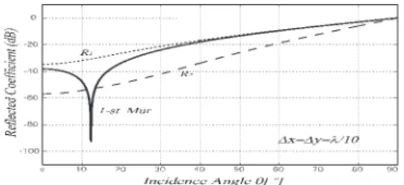
In Fig.4, theoretical reflection coefficients of these absorbing boundary conditions as a function ofincident angleθare shown. The cell size was set to be1/10per wavelength. It is found that the reflection coefficient at θ＝0 does not become zero due to the extrapolation approximation. Moreover, the reflection coefficient increases as the incident angle increases. Note that the accuracy of IEABC is greatly enhanced compared with the 1st Murs ABC. However, for EABC, the reflec-tion coefficient becomes as large as that of Murs ABC.

In Fig. 5, the reflection coefficients of ABCs are shown, where the cell size was set to be 1/20 per wavelength. Over a wide range of angles,the reflection coefficient of IEABC is smaller than that of 1st Murs ABC and EABC, except at the angle θ＝6 . However, the reflection of IEABC is −70 and sufficiently small enough. From this figure, the IEABC is superior to 1st Murs ABC in regard to high absorption ability for oblique incidence with arbitrary angle.

In Fig. 6, Fig. 7, and Fig. 8, the performance of the IEABC in the frequency domain by Eq. and that of Murs ABC［3］are shown for incident angleθ＝0 ,30 , and 60 , respectively, where the reflection coefficients

Figure 4:Reflection coefficient (solid:1st Mur,dotted: EABC, dashed: IEABC) of plane wave with oblique incident angle θ.

Figure 5: Reflection coefficient of plane wave with oblique incident angle θ.

Figure 6:Reflection coefficient of ABCs versus normal-ized frequency Δ (θ＝0 ).

Figure 7:Reflection coefficient of ABCs versus normal-ized frequency Δ (θ＝30 ).

Figure 8:Reflection coefficient of ABCs versus normal-ized frequency Δ (θ＝60 ).

are plottedas a function of normalized frequency Δ . In Fig. 6, the reflection coefficient of IEABC for θ ＝0 rapidly drops to − as Δ →0,compared with 1st Murs ABC,whereas both of these curves go to 0 for Δ → π, i.e., Δ ＝λ/2. Also, in Fig 8, it is shown that reflection coefficient of IEABC is smaller than that of 1st Murs ABC for all of the frequency range. However,in Fig.7,the reflection coefficient of 1st Murs ABC shows a minimum at Δ ＝π/2 and is smaller than that for IEABC around this frequency. In situations where accurate calculation of antenna impedance, radar cross sections, and so on is required, cell size should be chosen to be1/20 per wavelength or smaller. This means that the frequency range should be π/10 or lower. In this range, the reflection coeffi-cient of IEABC is smaller than that of 1st Murs ABC having a difference of over 20 . From the point of practical simulation, IEABC always shows a smaller reflection coefficient than 1st Murs ABC.

４ Numerical Example

In this section, we compare the magnitude of the reflected electric field employing IEABC with other absorbing boundary conditions［2］［3］.

First, we define the analysis region as200×200 cells in 2D free space［6］. The parameter Δ ＝Δ ＝2 Δ ＝ /60,where the input Gaussian pulse holds a peak at time ＝ as shown in Eq. ［5］.

＝exp −α − 0 2

The plane wave of Gaussian pulse is initially placed at the center ＋1₂, ＝100＋1₂ of the analysis region as . We calculate reflection of the TE wave propagating in the positive direction and incident normally on the absorbing boundary at ＝0 and ＝ 200.

Figure 9 empshows the electric field 100＋1/2,100 ＋1/2 using the absorbing boundaries of IEABC,Mur, and PML. The number of cells in PML layer is ＝ 16, and the reflection coefficient is set to be −150 . The electric conductivity profile is given as the fourth power of distance. The largest peak near 1.0［ns］is the incident wave. The electric field is normalized by the peak in the incident field. The peak near 4.5 and 7.5［ns］ show the first and second reflection from absorbing boundary ＝200 and ＝0, respectively. The solid line indicates the result of IEABC,by which the first reflection issuppressed as small as −115 .

The second reflection is completely absorbed in the vicinity of 7.5［ns］. Dotted and dashed lines depict the result of Murs ABC and PML with the first reflec-tion of−75 and −135 , respectively. However, for PML with 12 layers,the reflection becomes as large as that of IEABC. On the memory consumption,there is great advantage in the IEABC. The IEABC uses memory with respect to PML in 1D problems, because the IEABC absorbs by making use of one outermost one cell whereas PML needs cells. In the 2D case, the memory consumption is to PML. The EABC without improvement by Eq. shows the Figure 10: Relation between dielectric constants and

reflection characteristics (solid: ε＝3.0, dashed: ε＝ 9.0) in IEABC.

Figure 9: Comparison of reflection characteristics (solid:IEABC, dotted:Murs ABC, dashed:PML).

same degree of absorption as Murs ABC.

Since extrapolation is used with the assumption that the electromagnetic field changes linearly, accuracy increases with finer cell size as shown in Fig. 10. Under the same condition as in Fig.9,Fig.10 shows the reflection characteristicsfor a relative permittivity ε＝ 3.0 and ε＝9.0. The reflection characteristic of the absorbing boundary in a medium with high per-mittivityturns for the worse,because the number of cells per a wavelength becomes elatively smallin the medium.

In previous examples, we discussed reflection of the plane wave in free space. Now let us consider the reflection characteristics of a guided wave in the follow-ing. The dielectric slab waveguide considered in this example is shown in Fig. 11, and has the following parameters: ＝1λ 5λ, ＝1.5 and ＝1.49. We treat propagation of TE modes with the wavelength λ＝ 1.55μ . The computational region consists of × cells, with the maximum mesh numbers ＝400 and ＝1000. The outskirts are the absorbing boundaries of IEABC or PML. The increments are Δ ＝Δ ＝2 Δ ＝λ/60. The incident plane is at ＝ /2. As an example consider a continuous, monochromatic TE mode which propagated in the positive direction is launched from the incident plane. Here, we used an excitation method of positive propagating waveform［8］［9］.

In Fig. 11, we separate the computational region, with the incidence plane , into two sub regions;the total field region and the reflected field region. There-fore, an observer located in the reflected region should not detect any reflection, if no discontinuities exist in the total field region. For PML and EABC, instanta-neous field distributions at time step ＝6000 are shown in Fig. 12. To compare the amount of reflec-tion,we define normalized power by the numerical integration as follows:

＝∑_∑ ∑_∑ , .

Here, is index of grid with respect to -axis and is maximum grid number. The field is the input

electric field distribution of mode along the -axis. Time duration of ＝4800 6000 is for time average of the steady-state amplitudes. The power of the travel-ing and reflected wave at some points is shown in Table 1.

The power carried by the incident field to positive is set to unity,and also the power of the reflected wave should go to zero in analytical solutions. In this numerical analysis, error in the normalized power is Figure 11:Illustration of dielectric slab waveguide and computational region.

Figure 12:Instantaneous field distributions for ＝ 2λ. The distribution is recorded at time step ＝6000 and the contour lines are displayedfor each cell in 1

, /2−240 /2＋240. ⒜ PML with 12 layers, ⒝ IEABC.

limited to less than 0.32% of the incident power. In this situation the following three points are important: ⑴ the dispersion error,inherent in the FDTD method; ⑵ the error due to the parasitic wave in the source excitation;⑶ the reflected wave by absorbing boundary conditions. In this example,we can compare reflection characteristics with EABC and Berengers PML, as the effect at points⑴ and ⑵ are the same in both computa-tions. Figure 13 shows the difference in reflected power between EABC and PML. The reflection of IEABC becomes almost the same as that of 12 layers of PML in a slab waveguide, and we can obtain a quite small reflection characteristic by IEABC.

５ Conclusion

In this paper, the formulation and improvement of EABC for FDTD method is described. The reflection characteristic was compared with Murs ABC and Berengers PML. The IEABC showed better absorb-ing performance in comparison with Murs ABC, and the memory consumption is much smaller than PML. To obtain electromagnetic response over a long time period, the absorbing boundary with small reflection and small memory consumption is important from the points of view of accuracy and speed of computation. The proposed EABC is one of the most suitable tech-nique for this purpose.In a future study, we intend to use higher order extrapolation to obtain a much smaller amount of reflection.

REFERENCES

［１］K. S. Yee and J. S. Chen, Conformal hybrid finite difference time domain and finite volume time domain, IEEE Trans. Antennas Propagat.,vol.42, pp. 1450-1455, Oct. 1994.

［２］J.P.Berenger, A Perfectly Matched Layer for the Absorption of Electromagnetic Waves, J.Comput. Phys., vol. 114, no. 1, pp. 185-200, Oct 1994. ［３］G.Mur, Absorbing boundary Condition for the

finite-difference approximation of the time-domain electromagnetic-field equations, IEEE Trans. Electromagn. Compat., vol. EMC-23, no. 4, pp. 377-382, Nov 1981.

［４］K. Uchida, X. Li, H. Maeda and K. Y. Yoon, On Extrapolated Absorbing Boundary Condition for FVTD Method , Proc. of ISAP2005, Vol. 1, pp. 197-200, Seoul, Korea, Aug. 2005,

［５］T.Uno, Antenna Design Using the Finite Differ-ence Time Domain Method IEICE Trans.on Com-munications,Vol.E88-B No.5 pp.1774-1789,May, 2005.

［６］I.W. Sudiarta, An absorbing boundary condi-tion for FDTD truncacondi-tion using multiple absorbing surfaces , IEEE Trans. Antennas Propagat., vol. 51, no. 12, 3268-3275, December, 2003.

［７］Q. L., et al., Scattering by a two-dimensional periodic array of conducting plates, IEEE Trans. Antennas Propag., vol. 53, no. 12, pp. 4035-4042, Dec. 2005.

Figure 13:The difference of reflected powers between IEABC and PML.

Table 1:Normalized power of traveling and reflected wave evaluatedby Eq.

Location of observation plane

Reflected field Total field −20Δ −10Δ ＋10Δ ＋20Δ PML 0.000176 0.000176 1.002702 1.001844 ＝1λ EABC 0.000188 0.000189 1.001851 1.002695 PML 0.000171 0.000170 1.002715 1.001855 ＝2λ EABC 0.000186 0.000185 1.001447 1.003117 PML 0.000172 0.000171 1.002723 1.001861 ＝3λ EABC 0.000183 0.000182 1.001572 1.003005 PML 0.000172 0.000172 1.002728 1.001865 ＝4λ EABC 0.000181 0.000180 1.001782 1.002804 PML 0.000173 0.000173 1.002730 1.001867 ＝5λ EABC 0.000179 0.000179 1.001964 1.002626

［８］S. T. Chu, W. P. Huang and S. K. Chaudhuri, Simulation and analysis of waveguide based optical integrated circuits , Comp. Phys. Commun., vol. 68, pp. 451-484, 1991.

［９］W.P.Huang,S.T.Chu and S.K.Chaudhuri, A semivectorial finite-difference time-domain method , IEEE Photon. Technol. Lett., vol. 3, pp. 803-805, 1991.