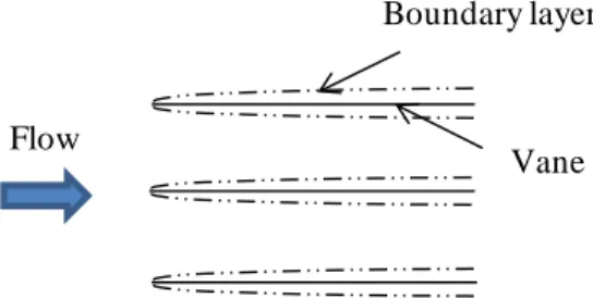
Boundary Layer Loss Reduction of Cascade Flow by Wide Chord
8
0
0
全文
図

+2

関連したドキュメント