Doctoral Dissertation
CONTINUOUS DISPLACEMENT MONITORING
BY USING GPS AND ITS APPLICATION TO A
LARGE-SCALE STEEP SLOPE
March, 2019
NGUYEN TRUNG KIEN
Graduate School of Sciences and Technology for Innovation
Yamaguchi University
© Copyright 2019 NGUYEN TRUNG KIEN
Continuous monitoring is very important for predicting the displacement behavior of slopes and for designing countermeasures against it. For instance, continuous monitoring is essential for large-scale steep slopes where the ground is likely to be unstable and great damage will be caused if the slopes collapse. It is known to be technically difficult to precisely and continuously monitor the displacement at such sites.
Recent studies have shown that the Global Positioning System (GPS) has the potential to continuously and precisely monitor displacements over extensive areas in civil and mining projects. Although GPS can measure three-dimensional displacements with mm accuracy for baseline lengths of less than 1 km, the measurement results include fatal errors due to obstructions above the antennas and tropospheric delays caused by weather conditions.
The objective of this research is to establish a method for precise slope monitoring by using GPS. The research includes
- Verification of the applicability of error-correction methods for reducing the influence of obstructions above the antennas and tropospheric delays at a large-scale steep slope for long-term monitoring;
- Discussion on the mechanism of the occurrence of large displacements of the slope due to an increase in the groundwater level by a numerical analysis based on the monitoring results;
- Investigation of the measurement performance of new GPS sensors, developed inexpensively compared with the current sensor, which can be installed at many points and can monitor displacements at any interval.
Chapter 1 describes the problem setting in this study and the organization of the dissertation, and Chapter 2 presents a literature review of GPS application for displacement monitoring together with an outline of GPS.
In Chapter 3, the applicability of error-correction methods for reducing the effects of obstructions above the antennas and tropospheric delays is investigated using GPS for displacement monitoring at a large-scale steep slope. As a result of applying the error-correction methods, the errors are reduced and/or eliminated from the
measurement results, and the measurement accuracy is improved. Thus, it is shown that monitoring results without errors can be obtained. Furthermore, the displacement results by GPS are compared with those by an extensometer and the Diffusion Laser Displacement Meter. It is found that the measurement sensitivity of the GPS displacement monitoring system is almost equivalent to that of the extensometer and the Diffusion Laser Displacement Meter.
Chapter 4 shows the results of long-term continuous monitoring at the slope using the error-correction methods described in Chapter 3. It is illustrated that the displacement could be continuously monitored with standard deviations of 1-2 mm in the horizontal direction and 3-4 mm in the vertical one without missing any data. During the measurement period, the groundwater level rose due to heavy rainfalls, the displacement greatly increased, and then parts of the slope were unstable in some cases. Thus, the mechanism of the occurrence of large displacements of the slope due to the increase in the groundwater level was investigated by numerical simulations based on the displacement monitoring results.
In the future, in order to conduct GPS monitoring more effectively, it will be necessary to install an inexpensive sensor at many points. In addition, it will also be essential to reduce the measurement interval from one hour to shorter intervals corresponding to the actual displacement behavior. New GPS sensors, which are capable of meeting such demands, are desired.
In Chapter 5, the measurement accuracy and the appropriate measurement intervals for the measurement performance by two new GPS sensors are investigated using the kinematic method. Fundamental experiments are conducted using the kinematic method with a 1-second measurement interval in which the baseline length and the height difference between the reference point and the observation point are changed. Standard deviations are improved by the arithmetic average of the 1-second kinematic results. Furthermore, experiments for detecting displacement are carried out. Field experiments with the new sensors are conducted at the slope discussed in Chapters 3 and 4.
Finally, Chapter 6 draws conclusions from the dissertation and discusses recommendations for future research works.
To
my father and mother
for their love and support.
Completing this PhD research has been one of the most challenging tasks in my life. However, it has also been an interesting journey in my life. During the PhD research, I received so much support and help from people around me, which has given me a chance to write these acknowledgements.
I would like to express my deepest gratitude to my supervisor, Prof. Norikazu Shimizu, and to my associate supervisor, Assoc. Prof. Shinichiro Nakashima, for their valuable guidance and continuous support in the course of my research. Their sharp and critical comments helped me to continuously improve not only my knowledge, but also the contents of my dissertation.
Thanks are also extended to Mr. Koji Kawamoto, Project Research Associate of the Shimizu Lab., for his help during much of this research, especially in field works. I also thank Mrs. Hitomi Uesaka and Mrs. Yoshie Furukawa, secretaries of the Shimizu Lab., for their assistance during my study in the Lab.
I also would like to thank the committee of my dissertation examination: Prof. Norikazu Shimizu, Prof. Toshihiko Aso, Prof. Yukio Nakata, Prof. Motoyuki Suzuki, and Assoc. Prof. Shinichiro Nakashima for their valuable advice and comments during the examination of this dissertation.
This research has been supported by JSPS KAKENHI (Grant-in-Aid for Scientific Research by the Japan Society for the Promotion of Science) [Grant Numbers 25350506 and 16H03153. Project leader: Prof. Norikazu Shimizu]. I am also grateful for the support that I received from the staff of Kokusai Kogyo Co., LTD, Japan for their support in sending the raw data on field monitoring. Thanks are also extended to Dr. Tomohiro Masunari, Kokusai Kogyo Co., LTD, and the staff of Nagata Electric Co., LTD for their help and discussions during this research in Chapter 5.
My sincere thanks also go to all of my Lab mates, especially former students of the GPS group at Yamaguchi University: Mr. Yuichiro Hayashi, Mr. Yota Furuyama, Mr. Shusaku Terada, Mr. Yuki Suma, and Mr. Hisamoto Awatsu; doctoral fellows: Mr. I Nyoman Sudi Parwata and Mr. Putu Edi Yastika; former students: Mr. Takashi Sakamoto, Mr. Shota Amafuji, Mr. Kento Okuda, Mr. Ryosuke Taguchi, Mr. Kei Sato, Mr. Yasunori Koga, Mr. Takeshi Ibara, Mr. Hayato Kurasaki, and Mr. Keita Imatani;
master students: Mr. Ryuto Yoshida, Ms. Akane Tochigi, Mr. Kentaro Yamato, Mr. Mitsuo Kameyama, Mr. Tokuma Ueno, Mr. Masaki Ozawa, and Mr. I Made Oka Guna Antara; and bachelor students: Mr. Rukiya Kiso for his support in field works, and Mr. Toru Shigetani, Mr. Seiichiro Komoto, Mr. Kosuke Shimai, Mr. Rei Kodama, Mr. Kaziki Shigehiro, and Ms. Shino Tsunemine for their friendship and warm kindness.
I also want to thank all of the Vietnamese and international students at Yamaguchi University for their support and for the happy times we shared together. Thanks are also extended to my host family, Mr. Masayuki Tsuruda and Mrs. Nobuko Tsuruda, for their support, encouragement, and the enjoyable days we had together.
I also would like to thank the International Student Office of Yamaguchi University, Ube International Student House Office, and Tokiwa Kogyo Society for their help and favors during my stay at Yamaguchi University and Ube City.
I acknowledge the Vietnam Ministry of Education and Training (MOET) and the Vietnam International Education Cooperation Department (VIED) for their financial support of my doctoral research at Yamaguchi University.
Thanks are also extended to members of the Division of Geotechnical Engineering, Faculty of Engineering, Thuyloi University (TLU), Vietnam for their advice and encouragement. Special thanks are also offered to Prof. Trinh Minh Thu, President of TLU, and Assoc. Prof. Hoang Viet Hung, Head of the Division of Geotechnical Engineering, TLU, Assoc. Prof. Bui Van Truong, Deputy Head of the Division of Geotechnical Engineering, TLU, for their support and encouragement.
Thanks are also extended to Ms. H. Griswold for proofreading this dissertation. Last, but not least, I would like to thank my parents, Mr. Nguyen Van Phuong and Mrs. Nguyen Thi Lan. I thank them for teaching me the value of education, the necessity of hard work, and sincerity. I am thankful to my sisters, Mrs. Nguyen Minh Trang and Ms. Nguyen Thi Thao, and my brother-in-law, Mr. Luong Nhu Cuong, for their encouragement and support during all these years. I offer my special thanks to my fiancée, Ms. Le Thi Mai Anh, for her patience and support. I also thank my other relatives for their encouragement.
This dissertation is hereby submitted to the Graduate School of Sciences and Technology for Innovation of Yamaguchi University as part of the requirements for the degree of Doctor of Engineering. The research described herein was conducted under the supervision of Prof. Norikazu Shimizu and Assoc. Prof. Shinichiro Nakashima of the Department of Civil and Environmental Engineering, Yamaguchi University. The manuscript is an original contribution by the author, except where acknowledgements and references are made to previous studies. Part of this work has already been presented in the publications given below.
1. Peer-reviewed journal paper
a. Shinichiro Nakashima, Yota Furuyama, Yuichiro Hayashi, Nguyen Trung Kien, Norikazu Shimizu, Seiichi Hirokawa. Accuracy enhancement of GPS displacements measured on a large steep slope and results of long-term continuous monitoring. Journal of the Japan Landslide Society 2018;55(1):13-24.
This paper presents the verification of the applicability of error-correction methods for reducing the influence of obstructions above antennas and tropospheric delays at a large steep slope. Furthermore, the GPS displacement monitoring system and the error-correction methods were applied for long-term monitoring of the displacement at the slope. The error-correction methods presented in this paper are included in Chapter 3 of this dissertation. The long-term monitoring results in this paper, together with recent monitoring results, are included in Chapter 4.
2. Peer-reviewed conference proceedings paper
a. Nguyen Trung Kien, Shinichiro Nakashima, Norikazu Shimizu. Mechanism of landslide behavior at an unstable steep slope based on field measurements and a numerical analysis: a case study. In: Proceedings of ARMS 10th Asian Rock Mechanics Symposium The ISRM International Symposium for 2018. Singapore; 2018.
This paper presents the displacement results at a large-scale steep slope monitored with GPS. Based on the monitoring results, it is seen that local collapses have occurred in some cases of the slope due to the increase in the groundwater level after rainfall events. Hence, the mechanism of the displacement behavior of the slope was investigated by considering both field measurements and numerical simulations. The results of this paper are included in Chapter 4 of this dissertation.
3. Non-peer-reviewed conference proceedings papers
a. Nguyen Trung Kien, Yuichiro Hayashi, Shinichiro Nakashima, Norikazu Shimizu. Long-term displacement monitoring using GPS for assessing the stability of a steep slope. In: Proceedings of the 2017 ISRM Young Sc
Symposium on Rock Mechanics (YSRM 2017 an ISRM Specialized Conference) and the 2017 International Symposium on New Developments in Rock Mechanics and Geotechnical Engineering (NDRMGE 2017). Jeju; 2017. p. 165 168.
This paper presents an outline of the GPS monitoring system and continuous displacement monitoring results using GPS at a large-scale steep slope. The results of this paper are included in Chapter 4 of this dissertation.
b. Nguyen Trung Kien, Yuichiro Hayashi, Shinichiro Nakashima, Norikazu Shimizu. Displacement monitoring using GPS for a steep and large slope. In: Proceedings of 37th West Japan Symposium on Rock Engineering. Yamaguchi; 2016. p. 83 90.
This paper provides an outline of the GPS monitoring system, the error-correction methods, and practical application for monitoring slope stability. The contents of this paper are included in Chapters 3 and 4 of this dissertation.
c. Nguyen Trung Kien, Shinichiro Nakashima, Norikazu Shimizu. Consideration of mechanism of landslide behavior at an unstable slope caused by changes of the groundwater level. In: Proceedings of 39th West Japan Symposium on Rock Engineering. Nagasaki; 2018. p. 36 39.
This paper describes the results of numerical simulations to understand the mechanism of the displacement behavior considering changes in the groundwater level. Part of this paper is included in Chapter 4 of this dissertation.
4. Extended abstract
a. Nguyen Trung Kien, Shinichiro Nakashima, Norikazu Shimizu. Mechanism of landslide behavior at an unstable slope caused by changes of the groundwater level. In: Proceedings of the 20th International Summer Symposium The 73rd Annual Conference of the Japan Society of Civil Engineers. Sapporo; 2018. This extended abstract describes the results of numerical simulations to understand the mechanism of the displacement behavior considering changes in the groundwater level. Part of this paper is included in Chapter 4 of this dissertation.
ABSTRACT i
ACKNOWLEDGMENTS iv
PREFACE vi
TABLE OF CONTENTS ix
LIST OF FIGURES xii
LIST OF TABLES xviii
LIST OF ACRONYMS xix
LIST OF SYMBOLS xx
Chapter 1 INTRODUCTION 1
1.1. General background 1
1.2. Problem statement 3
1.3. Objectives and scope of research 4
1.4. Organization of dissertation 5
Chapter 2 LITERATURE REVIEW AND OUTLINE OF GPS 7
2.1. Literature review 7
2.1.1. Conventional and recent displacement monitoring techniques 7 2.1.2. GPS application for displacement monitoring 9 2.1.2.1. Monitoring campaign and data acquisition 10
2.1.2.2. GPS processing methods 11
2.1.2.3. Accuracy of monitoring systems 12
2.1.2.4. Costs of monitoring schemes 13
2.2. Outline of GPS 14 2.2.1. GPS segments 14 2.2.2. GPS observables 15 2.2.2.1. Code pseudoranges 15 2.2.2.2. Phase pseudoranges 17 2.2.3. Coordinate systems 19
2.2.3.1. World Geodetic System 1984 (WGS84) 19
2.2.3.2. Transverse Mercator projection 20
Chapter 3 PROCEDURE TO ENHANCE THE ACCURACY OF DISPLACEMENT
MONITORING WITH GPS 23
3.1. Introduction 23
3.2. Outline of the system 23
3.3. Error sources and correction methods 24
3.3.1. General concept 24
3.3.2. Reduction of signal disturbances due to obstructions above antennas 25 3.3.3. Correction of tropospheric delays due to meteorological conditions 25 3.3.4. Estimation of exact values from measured results with random errors 27 3.4. Application of the procedure with the error-correction methods 28
3.4.1. Monitoring site 28
3.4.2. Original results 30
3.4.3. Effect of error correction for obstructions 31 3.4.4. Effect of error correction for tropospheric delays 35
3.4.5. Final results 38
3.5. Comparison with displacements by surface extensometer and Diffusion Laser
Displacement Meter 41
3.5.1. Surface extensometer 41
3.5.2. Diffusion Laser Displacement Meter (DLDM) 43
3.6. Chapter summary 44
Chapter 4 LONG-TERM CONTINUOUS MONITORING OF GROUND SURFACE
DISPLACEMENT AT A LARGE-SCALE STEEP SLOPE 46
4.1. Introduction 46
4.2. Continuous displacement monitoring 46
4.2.1. Site and monitoring points 46
4.2.2. Monitoring results 47
4.2.2.1. March 2013 to August 2014 47
4.2.2.2. August 2014 to January 2018 50
4.3. Mechanism of occurrence of large displacement at heavy rainfall 53
4.3.1. Problem setting 53
4.3.2. Numerical simulations 55
4.4. Chapter summary 62 Chapter 5 INVESTIGATION OF THE MEASUREMENT PERFORMANCE OF
THE NEW GPS SENSORS 64
5.1. Introduction 64
5.2. New sensors 64
5.3. Fundamental experiments 66
5.3.1. Baseline length: 10 m, height difference: 0 m 67 5.3.2. Baseline length: 200 m, height difference: 30 m 70
5.4. Experiments for detecting displacements 74
5.4.1. New GPS sensor SB-50S 74
5.4.2. New GPS sensor SB-35 76
5.5. Field experiments 78
5.5.1. Kinematic results 80
5.5.2. Interval of measurement time 82
5.6. Chapter summary 83
Chapter 6 CONCLUSIONS 84
6.1. Conclusions 84
6.2. Future research 86
Fig. 1.1. Flowchart of the dissertation ... 6
Fig. 2.1. GPS segments (adapted from Shimizu et al., 2014). ... 14
Fig. 2.2. GPS observation of a point based on code pseudoranges: ô ô and h are longitude, latitude, and height of the point above the reference ellipsoid; X, Y, and Z are the global geocentric Cartersian coordinates. ... 16
Fig. 2.3. Schematic of GPS carrier phase measurement. ... 17
Fig. 2.4. WGS84 reference frame (adapted from Misra and Enge, 2011). ... 19
Fig. 2.5. Transverse Mercator map projection (El-Rabbany, 2002). ... 20
Fig. 3.1. Schematic diagram of GPS displacement monitoring system (adapted from Nakashima et al., 2012b): (a) Sensor and (b) Monitoring system (Shimizu and Matsuda, 2002; Iwasaki et al., 2003; Masunari et al., 2003). ... 24
Fig. 3.2. Monitoring site and locations of GPS sensors (the dates below the GPS points indicate the monitoring period of the equivalent monitoring points). ... 29
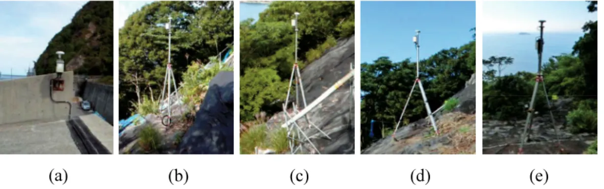
Fig. 3.3. Reference point K1 (a) and monitoring points G1 (b), G2 (c), G3 (d), and G4 (e). ... 29
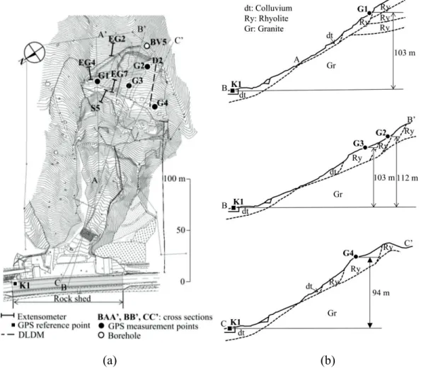
Fig. 3.4. Layout of locations of GPS sensors and extensometers on slope: (a) Plan view and (b) Vertical sections. ... 30
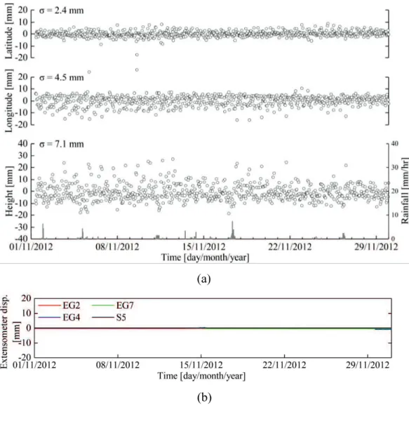
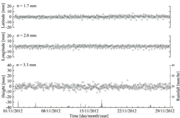
Fig. 3.5. Monitoring results at: (a) GPS (G1) without error correction from 1 November 2012 to 30 November 2012, (b) Extensometers (EG2, EG4, EG7, and S5) from 1 November 2012 to 30 November 2012, and (c) GPS (G1) without error correction from 7 November 2012 to 10 November 2012. ... 32
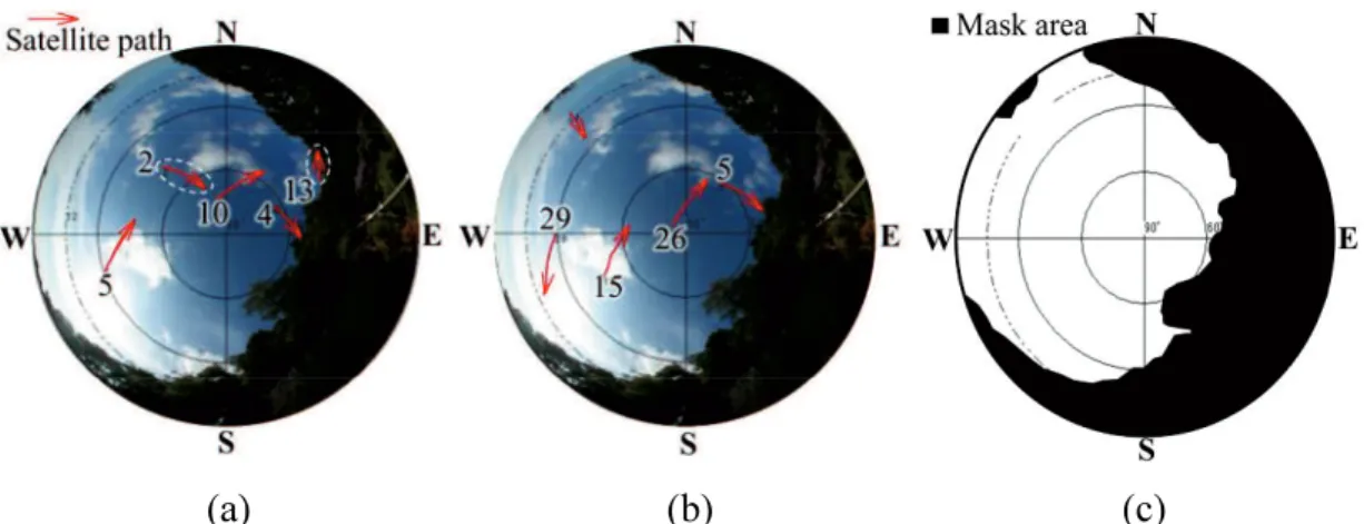
Fig. 3.6. Sky views and trace of satellite orbits above antenna at G1: (a) Period of scattered values (16:00 17:00 on 7 November 2012), (b) Period of normal values (19:00 20:00 on 7 November 2012), and (c) Mask area. ... 33
Fig. 3.7. Transition of residuals at G1 (16:00 - 17:00 on 07 November 2012): (a) Satellite 13 and (b) Satellite 2. ... 33
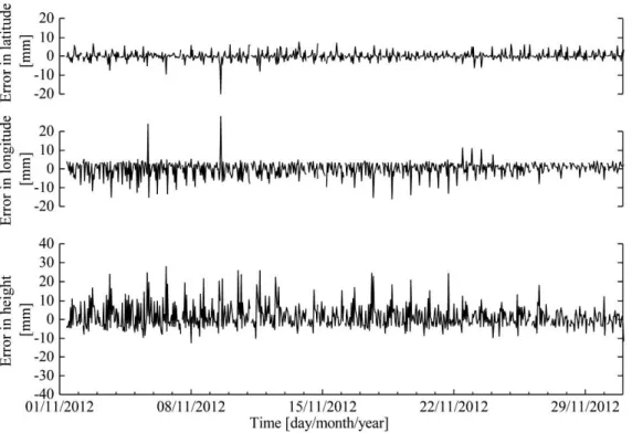
Fig. 3.9. Errors due to signal disturbances caused by obstructions above antenna, p.
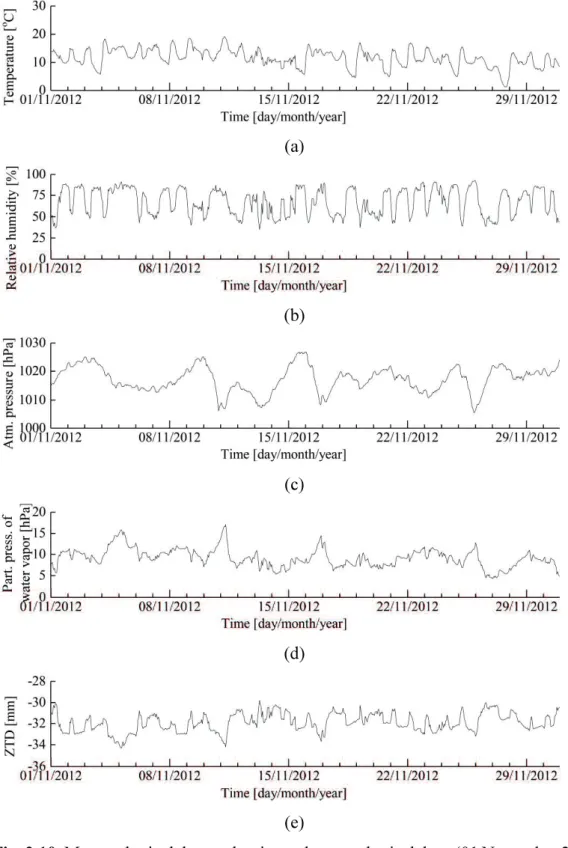
... 35 Fig. 3.10. Meteorological data and estimated tropospheric delays (01 November 2012 30 November 2012): (a) Temperature, (b) Relative humidity, (c) Atmospheric pressure, (d) Partial pressure of water vapor estimated by Eq. (3.9), and (e) Zenith tropospheric delay (ZTD) estimated by modified Hopfield model. ... 36 Fig. 3.11. Monitoring results at G1 after error correction by mask processing and tropospheric delay correction. ... 37 Fig. 3.12. Errors due to tropospheric delays, T. ... 37
Fig. 3.13. Monitoring results at G1 after applying the trend model with mask processing and tropospheric delay correction. ... 38 Fig. 3.14. Random errors, R. ... 39
Fig. 3.15. Fourier spectrum of height displacements at G1: (a) Without error correction, (b) With mask processing, (c) With mask processing and tropospheric delay correction, and (d) Applying the trend model with mask processing and tropospheric delay correction. ... 40 Fig. 3.16. Extensometer measurement EG-4 and GPS sensor at G1 (see Fig. 3.4). .. 42 Fig. 3.17. Comparison of displacements monitored by GPS and extensometer EG-4 (01 April 2013 01 January 2014). ... 42 Fig. 3.18. Comparison of displacements monitored by GPS and extensometer EG-4 at beginning of movement (01 June 01 October 2013). ... 42 Fig. 3.19. Diffusion Laser Displacement Meter (DLDM, see Fig. 3.4): (a) DLDM and (b) Reflector. ... 43 Fig. 3.20. Comparison of displacements monitored by GPS at G4 and DLDM (D2).
... 43 Fig. 4.1. Sky views above GPS antennas at: (a) G2, (b) G3, and (c) G4. ... 47 Fig. 4.2. Continuous three-dimensional displacement monitoring results (11 March 2013 to 12 August 2014). ... 48 Fig. 4.3. Displacement vectors at G1 and G2 (11 March 2013 to 12 August 2014
every 50 mm of the resultant displacement denoted by Plan view and (b) Vertical sections. ... 49
Fig. 4.4. Local failure around G1: (a) Situation on 28 January 2013 and (b) Situation on 31 August 2013 (adapted from Naya et al., 2014). ... 50 Fig. 4.5. Continuous three-dimensional displacement monitoring results (12 August 2014 to 26 January 2018). ... 51 Fig. 4.6. Displacement vectors at G2, G3, and G4 (12 August 2014 to 26 January 2018 Plan view and (b) Vertical sections. ... 52 Fig. 4.7. Displacement in direction of height at G2 with and without correction of mask processing and tropospheric delay correction. ... 53 Fig. 4.8. Continuous three-dimensional displacement monitoring results (May to October 2013). ... 54 Fig. 4.9. Displacement vectors at G1 and G2 (May to October 2013 every 50 mm of Plan view and (b) Vertical sections. ... 55 Fig. 4.10. UDEC model. ... 57 Fig. 4.11. Unbalanced force: (a) Initial equilibrium and (b) After the water level reaches point D. ... 58 Fig. 4.12. Relationship between changes in water pressure and displacements. ... 58 Fig. 4.13. Stress path at points 1, 2, and 3 on boundary between rhyolite and granite.
... 59 Fig. 4.14. Displacement distribution: (a) Case 1: hw = 127.5 m and (b) Case 2: hw = hd
= 127.6 m. ... 60 Fig. 4.15. Velocity vectors: (a) Case 1: hw = 127.5 m and (b) Case 2: hw = hd = 127.6 m. ... 61 Fig. 4.16. Displacement contours in Case 2: (a) X (horizontal) displacement and (b) Y (vertical) displacement. ... 62 Fig. 5.1. GPS sensors: (a) MG31 with flat antenna, (b) SB-50S with helical antenna and ground plane (Terada, 2017), and (c) SB-35 with Tallysman TW-1421 and 920 Mhz radio link. ... 65
Fig. 5.2. Schematic of experiments using SB-50S and SB-35 (adapted from Terada, 2017): (a) Fundamental experiments and (b) Experiment for detecting displacement. ... 65 Fig. 5.3. GPS sensors: (a) SB-50S and (b) SB-35. ... 66 Fig. 5.4. Measurement results by SB-50S (baseline length: 10 m, height difference: 0 m): (a) Post kinematic results with measurement interval of 1 second, (b) 1-minute average of kinematic results, (c) 5-1-minute average of kinematic results, (d) 10-minute average of kinematic results, (e) 20-minute average of kinematic results, (f) 30-minute average of kinematic results, (g) 60-minute average of kinematic results, and (h) Static analysis with 1-hour observation. ... 68 Fig. 5.5. Measurement results by SB-35 (baseline length: 10 m, height difference: 0 m): (a) Real-time kinematic results with measurement interval of 1 second, (b) 1-minute average of kinematic results, (c) 5-minute average of kinematic results, (d) 10-minute average of kinematic results, (e) 20-minute average of kinematic results, (f) 30-minute average of kinematic results, (g) 60-minute average of kinematic results, and (h) Static analysis with 1-hour observation. ... 69 Fig. 5.6. Measurement results by SB-50S (baseline length: 200 m, height difference: 30 m): (a) Post kinematic results with measurement interval of 1 second, (b) 1-minute average of kinematic results, (c) 5-1-minute average of kinematic results, (d) 10-minute average of kinematic results, (e) 20-minute average of kinematic results, (f) 30-minute average of kinematic results, (g) 60-minute average of kinematic results, and (h) Static analysis with 1-hour observation. ... 71 Fig. 5.7. Measurement results by SB-35 (baseline length: 200 m, height difference: 30 m): (a) Real-time kinematic results with measurement interval of 1 second, (b) 1-minute average of kinematic results, (c) 5-minute average of kinematic results, (d) 10-minute average of kinematic results, (e) 20-minute average of kinematic results, (f) 30-minute average of kinematic results, (g) 60-minute average of kinematic results, and (h) Static analysis with 1-hour observation. ... 72 Fig. 5.8. Relationship between average periods and standard deviations (baseline length: 10 m, height difference: 0 m): (a) SB-50S and (b) SB-35. ... 73 Fig. 5.9. Relationship between average periods and standard deviations (baseline length: 200 m, height difference: 30 m): (a) SB-50S and (b) SB-35. ... 73
Fig. 5.10. Slider to simulate displacement. ... 74 Fig. 5.11. Measurement results by SB-50S (10-mm given displacement in latitude): (a) Post kinematic results with measurement interval of 1 second, (b) 10-minute average of kinematic results, (c) 20-minute average of kinematic results, (d) 30-minute average of kinematic results, and (e) 60-30-minute average of kinematic results. ... 75 Fig. 5.12. Measurement results by SB-50S (5-mm given displacement in latitude): (a) Post kinematic results with measurement interval of 1 second, (b) 10-minute average of kinematic results, (c) 20- minute average of kinematic results, (d) 30-minute average of kinematic results, (e) 60-30-minute average of kinematic results. ... 75 Fig. 5.13. Measurement results by SB-35 (10-mm given displacement in longitude): (a) Real-time kinematic results with measurement interval of 1 second, (b) 10-minute average of kinematic results, (c) 20-10-minute average of kinematic results, (d) 30-minute average of kinematic results, (e) 60-minute average of kinematic results. ... 77 Fig. 5.14. Measurement results by SB-35 (2-mm given displacement in longitude): (a) Real-time kinematic results with measurement interval of 1 second, (b) 10-minute average of kinematic results, (c) 20-10-minute average of kinematic results, (d) 30-minute average of kinematic results, (e) 60-minute average of kinematic results. ... 77 Fig. 5.15. Monitoring site and locations of new GPS sensors. ... 78 Fig. 5.16. Reference points: (a) SB-50S-1 and (b) SB-35-1 (b); Observation points: (c) SB-50S-2 and (d) SB-35-2. ... 79 Fig. 5.17. Sky views and trace of satellite orbits above antennas at: (a) SB-50S-1, (b) SB-50S-2, (c) SB-35-1, and (d) SB-35-2. ... 79 Fig. 5.18. Measurement results by SB-50S (baseline length: 181 m, height difference: 100 m): (a) Post kinematic results with measurement interval of 1 second, (b) 1-minute average of kinematic results, (c) 5-1-minute average of kinematic results, (d) 10-minute average of kinematic results, (e) 20-minute average of kinematic results, and (f) 30-minute average of kinematic results. ... 80
Fig. 5.19. Measurement results by SB-35 (baseline length: 170 m, height difference: 91 m): (a) Real-time kinematic results with measurement interval of 1 second, (b) 1-minute average of kinematic results, (c) 5-minute average of kinematic results, (d) 10-minute average of kinematic results, (e) 20-minute average of kinematic results, and (f) 30-minute average of kinematic results. ... 81 Fig. 5.20. Relationship between average periods and standard deviations (field experiments): (a) SB-50S and (b) SB-35. ... 82
Table 2.1. Overview of surface displacement measuring techniques and their precision
(Gili et al., 2000). ... 8
Table 2.2. WGS84 fundamental parameters (Misra and Enge, 2011). ... 20
Table 3.1. Standard deviations. ... 34
Table 4.1. ... 47
Table 4.2. Standard deviations (11 March 2013 to 12 August 2014). ... 50
Table 4.3. Standard deviations (12 August 2014 to 26 January 2018). ... 51
Table 4.4. Mechanical properties of rock at studied slope. ... 56
Table 5.1. Specifications of new sensors. ... 65
Table 5.2. Experiment cases. ... 66
Table 5.3. Standard deviations (fundamental experiments). ... 73
Table 5.4. Detection of displacement (SB-50S). ... 76
Table 5.5. Detection of displacement (SB-35). ... 78
GPS GNSS ISRM EDM TDR DLDM SAR LOS DInSAR C/A-code P-code WGS84 DoD JGD2000 CR-InSAR ZTD DEM UDEC GWL RTK
Global Positioning System
Global Navigation Satellite System
International Society for Rock Mechanics and Rock Engineering Electronic Distance Meter
Time Domain Reflectometry
Diffusion Laser Displacement Meter Synthetic Aperture Radar
Line of Sight
Differential Interferometry Synthetic Aperture Radar Coarse/Acquisition-code
Precision-code
World Geodetic System 1984 Department of Defense
Japanese Geodetic Datum 2000
Corner Reflector Interferometric Synthetic Aperture Radar Zenith Tropospheric Delay
Distinct Element Method
Universal Distinct Element Code Groundwater level
Measured travel times of codes from four satellites
Measured code pseudoranges between the receiver and the satellites
Speed of light in vacuum 2.99792458 x 10⁸ m/s Unknown clock bias
Coordinates of satellites from navigation message transmitted from satellites
Unknown coordinates of receiver point
, , h Longitude, latitude, and height
Signal phase from satellite k to observation point mi Distance from satellite k to observation point mi
Ionospheric delay (error) of signal phase from satellite k to observation point mi
Tropospheric delay (error) of signal phase from satellite k to observation point mi;
Receiver mi clock bias (error) Satellite k clock bias (error) Wavelength of signal
Unknown integer ambiguity from satellite k to observation point
mi
Observation error of signal phase from satellite k to observation point mi
Double-phase difference between observation point mi and reference point mr for satellite k and l
a Semi-major axis
b Semi-minor axis 1/f Reciprocal flattening
f Inverse flattening
X, Y Northing, Easting Scale factor Latitude of origin Central meridian Meridian arc length
y Measurement value
u0 Exact value
p Error due to signal disturbance caused by obstruction above
antenna
T Error due to tropospheric delay R Random error due to receiver noise
Tropospheric delay
NTrop Refractivity
Dry component of tropospheric delay Wet component of tropospheric delay Refractivity of dry component
Refractivity of wet component
hd Height of dry component hw Height of wet component
h Height above surface
p Atmospheric pressure
e Partial pressure of water vapor
T Absolute temperature
RH Humidity
y'n Corrected measurement results with random errors un Estimates for exact values of displacements Dt Measurement interval
t Progressing time
Operator for finite difference
vn, Rn White noises with average value of 0, standard deviation of , and
observation error with standard deviation of . jkn Normal stiffness of discontinuity
jks Shear stiffness of discontinuity jfric Friction angle of discontinuity jcoh Cohesion of discontinuity jperm Permeability factor
ares Residual hydraulic aperture azero Aperture at zero normal stress
hw Groundwater height measured from level of slope toe on right-hand side
hd Discontinuity height measured from level of slope toe on right-hand side
1.1.
A landslide is of rock, earth or debris down a slope (Cruden, 1991). It is one of the most serious natural hazards in mountainous areas. It often occurs suddenly and causes a threat to human life, the economy, etc. Due to changes in climate, fast population growth, a rise in infrastructural construction, etc., the tendency and frequency of the occurrence of landslides have increased and reached alarming rates in many countries (Saito et al., 2014; Dou et al., 2015; Avila et al., 2016; Scaringi et al., 2018). Two relevant peculiarities of landslides are their widespread spatial distribution and their inclination to be highly influenced by both human and natural factors that induce changes in the slope and the controlling factors (Gutiérrez et al., 2010). Landslides are also characterized as being time-dependent (Flageollet, 1996; Qin et al., 2001). A natural slope that has been stable for many years may suddenly collapse due to changes in topography, groundwater flows, the loss of strength, etc. (Abramson et al., 2002). In general, these failures may not be very well understood until the failure actually occurs and brings about the necessity to consider them. According to Hoek et al. (2000), rock slope failures are geological events that are controlled by natural physical processes. Although many researchers have investigated various ways to predict future failures of slopes, attempting to understand the mechanism behind large-scale failures is still a challengeable task.
The quest to understand the displacement (deformation) behavior of a slope has resulted in the development of various slope monitoring techniques. On the other hand, monitoring data play an important role in assessing slope stability, in predicting future slope behavior, and in designing countermeasure works. The monitoring techniques are based on different types of sensors, for instance, remote sensing, photogrammetric, and geodetic sensors, as well as geotechnical instruments, etc. These methods can also be divided into conventional and more recent techniques. To monitor the evolution of landslides, especially active landslides, the method should provide the real-time
evolution of the displacement. Therefore, this dissertation considers an automatic displacement monitoring system that can be used in real-time applications.
Using satellite remote sensing techniques provides the potential for understanding the landslide processes and for detecting displacements with sub-centimeter accuracy (Yin et al., 2010). However, the temporal resolution is limited by the frequency of the satellites traveling over an actual area, and these techniques are limited to episodic applications.
Airborne photogrammetry is a method that compares pictures taken at different epochs in time (Chandler and Moore, 1989). Although it is effective for determining long-time slow-moving landslides, it has the same problem of being episodic. It is impossible to perform real-time monitoring with this technique.
Several geotechnical techniques have been conventionally employed to monitor the displacement of grounds and structures, etc. Extensometers are used to measure the changes in distance between two points. Inclinometers are applied to measure the slope of initially straight boreholes. Piezometers are used to measure pore water pressure, and tiltmeters are used to measure the deviation from a horizontal plane, etc. However, all these conventional geotechnical techniques can only be applied to limited areas.
The last group of techniques are geodetic; they can be divided into two subgroups, based and satellite-based systems. The first subgroup, the ground-based techniques, apply leveling instruments, total stations, laser scanners, etc., and can perform an episodic monitoring program. However, these techniques are not only very labor intensive, but they are also expensive to use, especially when high temporal resolution is required. Another drawback is that it is troublesome to perform absolute displacement analyses with them in cases where the distance to the fixed points is long, which often occurs in high-risk landslide areas. The second subgroup, the satellite-based systems, makes use of the available Global Navigation Satellite Systems (GNSS), such as GPS, GLONASS, GALILEO, etc. These systems show the potential to measure baselines with high accuracy over long distances and extensive areas without any demand for a line-of-sight between receivers in real-time.
1.2.
Landslides cause many problems to human life, property and constructed facilities, infrastructures, and the natural environment. Mitigation is an urgent task to reduce the effects of landslides. There are four basic strategies for mitigating a particular landslide (Smelser, 2014):
- Stabilization - Protection - Avoidance
- Maintenance and monitoring
This research will be focused on the aspect of monitoring. Various techniques for assessing slope deformation have been studied to facilitate the design of countermeasures and to understand the mechanism of slope behavior. The question arises as to which parameters are most significant (Dunnicliff, 1988). The measurements of pressure, stress, load, strain, and temperature are often influenced by the specific conditions within a very small zone or the location of the slope. On the other hand, these parameters are dependent on the local characteristics of the zone. Therefore, they may not represent the conditions on a larger scale. In the case of requiring a large number of measurement points before confidence can be placed in the data, displacement (deformation) measurements can be meaningful and reliable. In addition, displacement monitoring is often the simplest way to examine the evolution of slope failure. Hence, displacement is chosen as the parameter for monitoring in this research.
The Global Positioning System (GPS) is a satellite-based positioning system. Nowadays, GPS is widely used to monitor the deformation of grounds and structures. Moreover, it is recognized that the GPS monitoring system can provide three-dimensional displacements with mm accuracy over extensive areas.
On the other hand, the GPS measurement results are generally scattered due to various error sources. To guarantee the reliability of the measurement results, some appropriate methods should be applied to reduce and/or eliminate the errors included in the measurement results. The errors due to tropospheric delays can be corrected by using an appropriate tropospheric delay model, like the modified Hopfield model
(Masunari and Shimizu, 2007; Masunari et al., 2009; Shimizu et al., 2011, 2014; Nakashima et al., 2012b). In addition, the errors due to obstructions above the antennas can be reduced by an analysis performed without the data taken from the satellites moving behind the obstructions (Masunari et al., 2008; Shimizu, 2009; Shimizu et al., 2011, 2014). The random errors arising from random fluctuations can be removed by the application of an adequate method (Shimizu, 1999; Shimizu et al., 2014). These separated error-correction methods are also written in the ISRM Suggested Method for monitoring rock displacements using the Global Positioning System (GPS) (Shimizu et al., 2014) as suggestions for use with GPS monitoring. The question arises as to how the three separated error-correction methods can work together to improve the GPS measurement results, for example, when using GPS monitoring at a large-scale steep slope where the errors due to obstructions above the antennas and tropospheric delays occur at the same time. It is essential to apply a procedure with error-correction methods to enhance the accuracy of the measurement results for high precision monitoring when using GPS.
Another question is how to use the GPS measurement results for assessing the displacement behavior of a slope. On the other hand, the interpretation and the mechanism of the displacement behavior based on field measurements should be discussed.
In addition, the GPS sensors and the monitoring system are still expensive compared to standard geotechnical instruments (e.g., extensometers). In order to conduct GPS monitoring more effectively, sensors should be installed at many points and should be able to monitor the displacement at any interval. New sensors which can cope with these demands are desired. An investigation of the measurement performance with new GPS sensors should be conducted.
- Verification of the applicability of the error-correction methods for reducing the influence of obstructions above the antennas and tropospheric delays at a large-scale steep slope for long-term monitoring;
- Discussion on the mechanism of the occurrence of large displacements of the slope due to an increase in the groundwater level by a numerical analysis based on the monitoring results;
- Investigation of the measurement performance of new GPS sensors, developed inexpensively compared with the current sensor, which can be installed at many points and can monitor displacements at any interval.
1.4.
The dissertation is divided into six chapters. The flowchart of the dissertation is shown in Fig. 1.1. The content of each chapter is presented as follows:
Chapter 1 provides an introduction to the problem of slope failure, the background, the problem statement, the research objectives and scope of displacement monitoring for steep slopes, and the organization of the dissertation.
Chapter 2 presents a literature review of the conventional and the recent techniques for displacement monitoring. Furthermore, the application of GPS for displacement monitoring is reviewed together with an outline of GPS.
Chapter 3 investigates the applicability of the error-correction methods for reducing the effects of obstructions above the antennas and tropospheric delays when
using GPS for displacement monitoring at a large-scale steep slope. A procedure with error-correction methods to enhance the accuracy is proposed, and its applicability is verified for improving the GPS measurement results at a large-scale steep slope. Furthermore, the validity of the procedure is shown by a comparison between the displacement results by GPS and those by an extensometer and the Diffusion Laser Displacement Meter.
Chapter 4 shows the application of the GPS displacement monitoring system and the proposed procedure for long-term continuous monitoring at the large-scale steep slope. The interpretation of the displacement results is shown in plan views and vertical sections for assessing the time-evolution of the displacement behavior. Furthermore, the mechanism of the occurrence of large displacements at the slope due to the increase in the groundwater level was investigated by numerical simulations based on the displacement monitoring results.
Chapter 5 investigates the measurement performance of new GPS sensors using the kinematic method. Fundamental and field experiments are conducted to obtain the standard deviations of the new GPS sensors. The arithmetic average of the kinematic results is obtained when using the new GPS sensors.
Chapter 6 draws conclusions from the research presented within this dissertation and proposes recommendations for future research works.
Fig. 1.1. Flowchart of the dissertation
CHAPTER 1 INTRODUCTION CHAPTER 2 LITERATURE REVIEW AN OUTLINE OF GPS CHAPTER 3 PROCEDURE TO ENHANCE THE ACCURACY OF DISPLACEMENT
MONITORING WITH GPS
CHAPTER 5
INVESTIGATION OF THE MEASUREMENT PERFORMANCE OF THE NEW GPS
SENSORS
CHAPTER 6 CONCLUSIONS CHAPTER 4
LONG-TERM CONTINUOUS MONITORING OF GROUND SURFACE DISPLACEMENT
Monitoring techniques are used to observe and analyze the displacements of slopes and the conditions that trigger them, and they provide information for designing countermeasures, etc. Hence, it would also be beneficial to understand the monitoring techniques. Herein, a literature review of the conventional and recent techniques for displacement monitoring are presented. Furthermore, a review of GPS applications for displacement monitoring is also presented together with an outline of GPS.
2.1.
2.1.1. Conventional and recent displacement monitoring techniques
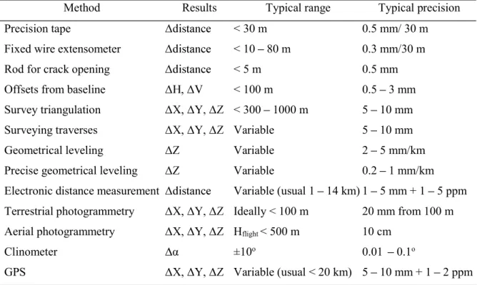
There are various displacement monitoring techniques that can provide the evolution of slope displacement over time, the responses to triggering conditions, and useful information for designing countermeasures, etc. The monitoring techniques involve periodic and automatic measuring. The evolution of the displacement at a steep slope can be understood by using many types of sensors. Geotechnical engineers have the important task of determining which sensors will provide the best description of the deformation. Gili et al. (2000) summarized the main techniques for measuring surface displacements and their degrees of precision (Table 2.1).
Several types of monitoring techniques have been developed and applied to measure ground movements in unstable areas. Precision tape and wire devices have been applied to measure changes in the distance between points or crack walls (Dunnicliff, 1984; Gulla et al., 1988; Brückl et al., 2013). Inclinometers have been applied to detect the depth of shear movement. This depth is also the depth of the failure surface (Slope Indicator, 2011). Tiltmeters have been used to perform rapid and precise measurements (Wyllie and Mah, 2004). Ashkenazi et al. (1998) used levels, theodolites, Electronic Distance Meters (EDM), and a total station to measure coordinates and changes in targets, control points, and landslide features. Aerial and terrestrial photogrammetry are convenient tools that have been employed to make
contour maps and to find the cross sections and point coordinates of landslide areas. In addition, photogrammetric compilation has proven useful for analyzing the changes in slope morphology and for determining the movement vectors (Ballantyne et al., 1988; Chandler and Moore, 1989; Oka, 1998). The advantages of these conventional techniques are that they are able to obtain precise measurements. However, they only provide one-dimensional displacements and they can only be applied to measure local areas. In other words, these conventional techniques are not suitable for landslide covering in high-altitude mountainous zones or extensive areas. Furthermore, it is difficult to collect data automatically and continuously in real-time at large-scale steep slopes with these techniques.
Table 2.1. Overview of surface displacement measuring techniques and their precision (Gili et al., 2000).
Method Results Typical range Typical precision
Precision tape
Fixed wire extensometer Rod for crack opening Offsets from baseline Survey triangulation Surveying traverses Geometrical leveling Precise geometrical leveling Electronic distance measurement Terrestrial photogrammetry Aerial photogrammetry Clinometer GPS < 30 m < 10 80 m < 5 m < 100 m < 300 1000 m Variable Variable Variable Variable (usual 1 14 km) Ideally < 100 m Hflight < 500 m ±10o Variable (usual < 20 km) 0.5 mm/ 30 m 0.3 mm/30 m 0.5 mm 0.5 3 mm 5 10 mm 5 10 mm 2 5 mm/km 0.2 1 mm/km 1 5 mm + 1 5 ppm 20 mm from 100 m 10 cm 0.01 0.1o 5 10 mm + 1 2 ppm
Recently, new technologies have been used to monitor slopes such as the Global Positioning System (GPS), Time Domain Reflectometry (TDR), the Diffusion Laser Displacement Meter (DLDM), and Synthetic Aperture Radar (SAR). With TDR, the depth to a shear plane or shear zone in a landslide can be located. However, TDR cannot determine the actual magnitude or direction of movement (Cortez et al., 2009). TDR can only detect the shear plane or shear zone. Moreover, if water infiltrates a
TDR cable, it will change the electrical properties of the coaxial cable. This may make it difficult to interpret the results.
The DLDM was developed by Naya et al. (2008, 2014) for monitoring rock/ground displacements. It can detect displacements of at least 1-2 mm for a baseline length of 62.5 m under rainfall intensities up to 120 mm/hr and displacements of at least 1-2 mm for a baseline length of 30 m even under rainfall intensities up to 200 mm/hr. The DLDM is similar to extensometers and inclinometers in that it can only observe the displacement in one-dimension.
Synthetic Aperture Radar (SAR) is a form of radar used to capture two- or three-dimensional images of objects. It can detect the displacement components along the sensor target line of sight (LOS) with high precision. The differential SAR interferometry (DInSAR) technique is employed for monitoring the small-scale movements on the surface. The accuracy of DInSAR is in the order of sub-centimeters. However, the drawbacks of DInSAR are geometric and temporal decorrelation, as well as atmospheric disturbances (Perissin and Wang, 2011).
2.1.2. GPS application for displacement monitoring
Conventional displacement monitoring techniques are limited to use in small areas and can measure only one-dimensional displacements. In addition, these conventional techniques are difficult and dangerous to install at large-scale steep slopes. The drawbacks of recent techniques, such as TDR, the DLDM, and DInSAR, are the inability to determine the actual magnitude and direction of movement, observing displacements in only one-dimension, and temporal decorrelation, respectively.
Nevertheless, the Global Positioning System (GPS), a displacement monitoring system, shows the potential to overcome the limitations of the above techniques. This research, therefore, employs the GPS technique for displacement monitoring.
GPS was established as a method for navigation and long baseline surveys (Hofmann-Wellenhof et al., 2001; Misra and Enge, 2011). It was first used for displacement monitoring in the mid-1980s in the fields of civil and mining engineering and other related fields (Burkholder, 1988, 1989; Chrzanowski and Wells, 1988).
Since then, many researchers have used GPS in practical applications (Stewart and Tsakiri, 1993; Behr and Hudnut, 1998; Gili et al., 2000; Malet et al., 2002; Kim et al., , and preliminary guidelines have been published for displacement (deformation) monitoring (US Army Corps of Engineers, 2002; Vermeer, 2002; Bond, 2004).
Recently, GPS techniques have been widely used to monitor the ground (Ma et al., 2012), slopes (Shimizu and Nakashima, 2017), and dams (Nakashima et al., 2012a), etc. Some studies have used GPS for displacement monitoring and have compared the results from conventional techniques, such as theodolite, electronic distance measurement, levels, total station, inclinometers, and wire extensometers (Gili et al., 2000; Moss, 2000; Malet et al., 2002; Rizzo, 2002; Coe et al., 2003; Tagliavini et al., 2007; Bertacchini et al., 2009; Calcaterra et al., 2012). Other studies have combined GPS and other surveying techniques, for example, terrestrial laser scanning, SAR interferometry, CR-InSAR, and photogrammetry for landslide investigations (Mora et al., 2003; Rott and Nagler, 2006; Peyret et al., 2008; Yin et al., 2010; Wang, 2011; Zhu et al., 2014). These integrations have provided useful information on displacements, magnitude, direction, evolution, etc. Based on the above studies, it is now recognized that the GPS monitoring system can provide three-dimensional displacements with mm accuracy over extensive areas.
Furthermore, the GPS displacement monitoring system can be classified by a number of factors, namely, automation, enhancement accuracy, etc. (Szostak-Chrzanowski and (Szostak-Chrzanowski, 2008). Based on the scope of this research, those factors related to displacement monitoring using GPS are reviewed.
2.1.2.1.Monitoring campaign and data acquisition
GPS displacement monitoring has been performed by both periodic (Rawat et al., 2011; Wang, 2012) and continuous (Masunari et al., 2003; Wang et al., 2012; Xiao et al., 2012) monitoring campaigns. The choice of a particular monitoring campaign depends on the critical factors of accuracy, cost, and safety of the equipment, etc.
On the other hand, in the standard method for monitoring displacements with GPS, it is required that a survey team revisit the monitoring site at regular intervals, for example, every few weeks or months. The static, rapid static or real-time kinematic
GPS surveying techniques can be used to construct a time series of the displacements observed at the monitoring points.
The main advantage of the standard method is that it requires a lower initial cost. One set of GPS equipment can be used to monitor several locations of a slope. Furthermore, the GPS equipment can also be used for other surveying purposes when it is not being used for displacement monitoring.
However, there are some disadvantages in using the standard method. The lower precision and poorly represented samples from the time series are two main disadvantages of this method. In this method, ground marks are used as monumentations. Setup errors can also occur in this method. It is often required that many points be observed in a short period of monitoring time. The coordinate precision is low as a result of the short observation times. Furthermore, the discontinuous time series is another disadvantage. The short period observations are often not enough to adequately grasp the trend of the displacement.
When standard receivers are employed for monitoring displacements, the GPS data are downloaded manually from the receivers. Then, data processing is conducted to obtain the coordinates of the monitoring points and to calculate the displacements for each session. This is inconvenient and ineffective for continuous monitoring.
To overcome the above limitations of the standard method, an automatic monitoring system that was previously developed (Shimizu and Matsuda, 2002; Iwasaki et al., 2003; Masunari et al., 2003) is employed in this study. The automatic monitoring system requires the following items (Iwasaki et al., 2003):
System stability for long-term monitoring High accuracy of the measurements
Quick data acquisition, analysis, and evaluation for many slopes at once Rapid notification of the monitoring results to the clients
Low cost
2.1.2.2.GPS processing methods
GPS displacement monitoring systems are classified based on how the system processes, utilizes, and handles the GPS observation data. The first method is post-processing in which all the observations are processed by means of the least squares
method to obtain a set of coordinates. Then, some software packages are used to perform the displacement analysis. One of examples of this post-processing method is Leica GEOMoS (Leica Geosystems, 2009). This method has a small delay in the early detection of failure.
The second method utilizes position solutions by a real-time kinematic (RTK) mode to perform the displacement analysis (Shimizu et al., 1996, 1997). Another example of this processing method is used in the GOCA system (Kälber and Jäger, 2001; Jäger and González, 2006). The third method involves the simultaneous transmission of the raw data that have been acquired at all the GPS stations to the server computer. Then, the calculations are performed. GRAZIA (Gassner et al., 2002) is software that follows this approach.
The goal of this research is to conduct continuous displacement monitoring by GPS and to describe its application at a large-scale steep slope. A system that consists of GPS sensors, data-links between them, and a server computer, etc. was developed (Shimizu and Matsuda, 2002; Iwasaki et al., 2003; Masunari et al., 2003). An outline of the system will be given in Chapter 3.
2.1.2.3.Accuracy of monitoring systems
Accuracy plays an important role in any displacement monitoring system (Brown et al., 2006). To achieve displacement monitoring with high precision, many studies have been made on the modeling components of the GPS measurement results, such as models for tropospheric delays (Saastamoinen, 1972; Niell, 1996), etc. On the other hand, tropospheric delays, one of the bias errors, are obtained by using average parameters from numerical weather predictions together with time and approximate coordinates (Leandro et al., 2006; Lagler et al., 2013). Unfortunately, the wet delay component in the tropospheric delays depends on the water vapor content. The water vapor changes over time and space. Therefore, the above models are insufficient for achieving monitoring with high precision.
A correction method using the modified Hopfield model together with meteorological conditions observed at the monitoring site was proposed for correcting tropospheric delays (Masunari and Shimizu, 2007; Masunari et al., 2009; Shimizu et
al., 2011, 2014; Nakashima et al., 2012b). This correction method was proven effective for improving the measurement accuracy.
Another source of bias errors is caused by obstructions above antennas (Shimizu et al., 2014). Furthermore, the number of satellites that are observed by the receiver also affects the measurement accuracy (Koo et al., 2017). The analysis of data without the data from the satellites moving behind the obstructions is effective for reducing these errors and for improving the accuracy (Masunari et al., 2008; Shimizu, 2009; Shimizu et al., 2011, 2014).
Furthermore, it is recommended that random errors, caused by random fluctuations, be reduced by an adequate method (Shimizu et al., 2014). A trend model can yield good estimates from the original measurement results (Shimizu, 1999; Shimizu et al., 2014).
In order to achieve monitoring with high precision, especially at large-scale steep slopes where there are simultaneously obstructions above the antennas and a difference in height between the reference point and the monitoring points, a procedure with error-correction methods to enhance the measurement accuracy is proposed in this research for improving the measurement results. The detailed procedure is shown in Chapter 3.
2.1.2.4.Costs of monitoring schemes
GPS is now recognized as useful technology for monitoring extensive areas and large structures. It has the potential to measure three-dimensional displacements with mm accuracy for baseline lengths of less than 1 km. In order to conduct GPS monitoring more effectively, a sensor should be installed at many points and should be able to monitor displacement at any interval. Unfortunately, if GPS receivers are employed to monitor a huge area, such as dams and landslides, the investment costs are very high. In recent years, many researchers have been working on low-cost GPS receivers in an attempt to find a more economical solution to displacement monitoring using GPS. In particular, some studies have investigated the accuracy of low-cost single-frequency GPS receivers (Janssen and Rizos, 2003; Squarzoni et al., 2005). Other studies have also used low-cost GPS receivers in post-processing (Dabove et al., 2014; Cina and Piras, 2015), in near real-time (Eyo et al., 2014), and in real-time
approaches to monitoring landslide behavior. Furthermore, Zhang and Schwieger (2017) investigated the performance of the L1-optimized choke ring ground plane for a low-cost GPS receiver system. The performance of low-cost GPS receivers has also been investigated through the use of free and open source software, such as RTKLIB (Takasu and Yasuda, 2009; Bellone et al., 2014; Biagi et al., 2015, 2016) and goGPS (Biagi et al., 2015, 2016). Schrader et al. (2016) combined multiple consumer-grade GPS receivers to present an inexpensive way to achieve a better GPS performance. In addition, an automatic low-cost GPS monitoring system using WLAN communication has been introduced (Günther et al., 2008; Zhang et al., 2012). These studies show that low-cost GPS receivers have the potential to provide centimeter or sub-centimeter accuracy.
In the research within this dissertation, the measurement performance of new GPS sensors, being developed by a collaboration of the Shimizu Lab. (Yamaguchi University) and a manufacturer, is also investigated by experiments and field experiments using the kinematic method.
2.2.
2.2.1. GPS segments
Fig. 2.1. GPS segments (adapted from Shimizu et al., 2014). Space segment
The Global Positioning System (GPS) is a satellite-based positioning system. There are three different segments in the GPS, namely, the space segment, the control segment, and the user segment (Fig. 2.1). The space segment provides global coverage with observable satellites above elevations of 15o (Hofmann-Wellenhof et al., 2001). The satellites move in nearly circular orbits with an altitude of approximately 20200 km above the earth in a period of about 12 sidereal hours. The constellation currently contains 31 of these satellites. A platform for radio transceivers, atomic clocks, computers, and various ancillary equipment is provided by the GPS satellites to operate the system. Atomic clocks precisely control all the signal components to The control segment comprises a master control station, worldwide monitor stations, and ground control stations. The control segment tracks the satellites for the orbit, clock determination, prediction modeling, time synchronization of the satellites, and upload of the data message to the satellites. The user segment consists of the user equipment for either the military or civilians. The receivers are characterized by the observables (i.e., code pseudoranges or carrier phase) and the codes (i.e., C/A-code or P-code). The signals are provided by the satellites which track them simultaneously.
2.2.2. GPS observables
The GPS observables are differential ranges from the measured time or phase between the received signals and receiver-generated signals. The position of the user receiver can be obtained by determining the distances (ranges) from it to the satellites. These distances can be calculated with code pseudoranges or the carrier phase. Satellites and receiver clocks are used for the calculations. Doppler observations are not used in this dissertation. Hence, they are not mentioned any further.
2.2.2.1. Code pseudoranges
The code range method is used to measure the amount of time shift required to align the C/A-code replica, generated at the receivers, with the signals received from the satellites (Misra and Enge, 2011). Then, the time is multiplied by the speed of light in a vacuum to compute the distance. Since the satellite and the receiver clocks are not
synchronized, a small delay needs to be added to the time on the receiver clock (clock bias) (Fig. 2.2). At least four satellites are used to determine the four unknowns, X, Y,
Z, and the receiver clock delay. Eq. (2.1) shows the equations used to obtain the
coordinates of an observed point. The precision of this procedure is low due to the large distance between the satellites and the antennas. Hence, it is not suitable for high-precision surveying such as that required for landslide monitoring.
(2.1)
where: : measured travel times of the codes from four satellites;
: measured code pseudoranges between the receiver and the satellites; : speed of light in a vacuum 2.99792458 x 10⁸ m/s;
: unknown clock bias;
: coordinates of the satellites from the navigation message transmitted from the satellites.
: unknown coordinates of the receiver point.
Fig. 2.2. GPS observation of a point based on code pseudoranges: , , and h are longitude, latitude, and height of the point above the reference ellipsoid; X, Y, and Z are the global geocentric Cartersian coordinates.
Ð ø ÷ ±® ø , , h) ï
î
í
2.2.2.2. Phase pseudoranges
Fig. 2.3. Schematic of GPS carrier phase measurement.
In contrast, much more precise measurements can be achieved with millimeter accuracy by carrier phase measurements. The carrier phase method measures the phase difference between the carrier signal, generated by the receiver, and the carrier received from a satellite (Misra and Enge, 2011). Fig. 2.3 shows a schematic of the GPS carrier phase measurement. However, the carrier phase measurement remains fixed at a fraction of a cycle. The distance between the receiver and a satellite can be calculated by an unknown number of whole cycles plus the measured fractional cycle. This result is referred to as integer ambiguity. Complicated algorithms are required to achieve the solution (single, double, and triple differencing).
Methods to correct the various errors (i.e., tropospheric delays and ionospheric delays) and to resolve the integer ambiguities are applied to obtain accurate position estimates. Eq. (2.2) shows the basic equation including errors.
(2.2)
where:
- : signal phase from satellite k to observation point mi; Reference point
Observation point satellite k
- : distance from satellite k to observation point mi;
- : ionospheric delay (error) of signal phase from satellite k to observation point mi;
- : tropospheric delay (error) of signal phase from satellite k to observation point mi;
- : speed of light in a vacuum 2.99792458 x 10⁸ m/s; - : receiver mi clock bias (error);
- : satellite k clock bias (error); - : wavelength of the signal;
- : unknown integer ambiguity from satellite k to observation point mi; - : observation error of signal phase from satellite k to observation point mi.
The single-phase difference between observation point mi and reference point
mr for satellite k, , is calculated. Similarly, the single-phase difference for
satellite l, , is also calculated. The double-phase difference, , is obtained as follows:
(2.3)
Eq. (2.3) shows the fundamental equation for relative positioning. The biases of the receiver clock and the satellite clock are eliminated by using the double-phase difference process. Furthermore, when the baseline length between the observation point and the reference point is short, less than a few km in length, the ionospheric delay is also eliminated (Shimizu et al., 2014). The tropospheric delay remains when the height difference between the observation point and the reference point is a few tens of meters.
The double-phase difference is calculated from the observed phase by a GPS receiver. Then, the three-dimensional coordinates of the observation point and integer ambiguity, and , are determined by means of the least squares method for the residual, .
2.2.3. Coordinate systems
The position of a receiver can be expressed in a coordinate system that is fixed to the earth and moves with it (Misra and Enge, 2011). Based on the scope, this subsection presents an outline of the World Geodetic System of 1984 (WGS84) that is widely used around the world. The study site in this research is located in Yamaguchi Prefecture, Japan. Therefore, in order to obtain the displacements, the conversion from WGS84 to the local coordinate system, Transverse Mercator (Japan zone 3), is also conducted.
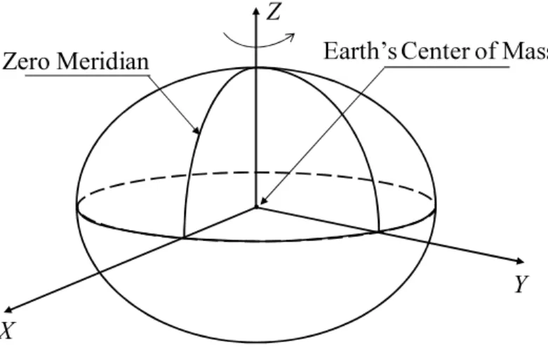
2.2.3.1. World Geodetic System 1984 (WGS84)
WGS84 is a 3-D, earth-centered reference system that was developed by the Defense Mapping Agency of the U.S. (Fig. 2.4), Department of Defense (DoD) (Misra and Enge, 2011). It is the official reference system for all mapping, charting, navigation, and geodetic products to be used throughout the DoD. WGS84 includes a coherent set of global models and definitions:
An earth-centered, earth-fixed Cartesian coordinate frame
An ellipsoid of revolution as a geometric model of the shape of the earth A characterization of the
A consistent set of fundamental constants
Fig. 2.4. WGS84 reference frame (adapted from Misra and Enge, 2011).
X
Y Z
Table 2.2. WGS84 fundamental parameters (Misra and Enge, 2011).
Parameter Value
Ellipsoid
Semi-major axis (a) Reciprocal flattening (1/f) Earth s angular velocity ( )
GM)
Speed of light in a vacuum (c)
6378137.0 m 298.25223563
7292115.0 x 10-11 rad/sec 3986004.418 x 108 m3/s2 2.99792458 x 10⁸ m/s
The user will refer to the position of a point in WGS84 as WGS84 LLA (for latitude, longitude, and altitude), or WGS84 XYZ coordinates. The positions of the GPS satellites are expressed in WGS84. The receiver positions, therefore, are obtained as WGS84 coordinates. The WGS84 is defined by fundamental parameters (Misra and Enge, 2011), as shown in Table 2.2.
2.2.3.2. Transverse Mercator projection
Transverse Mercator projection, known as Gauss-Krüger projection, is based on projecting the points on the ellipsoidal surface mathematically onto an imaginary transverse cylinder (El-Rabbany, 2002). The cylinder can be either a tangent or a secant to the ellipsoid (Fig. 2.5).
Fig. 2.5. Transverse Mercator map projection (El-Rabbany, 2002).
In Japan, the Japanese Geodetic Datum 2000 (JGD2000) was introduced as the geodetic reference system (Geographical Survey Institute, 2004). The monitoring site
Parallel Meridian Equator
X Y
Imaginary transverse cylinder Central meridian
in this research is located in Yamaguchi Prefecture, Japan where the origin of zone 3 in the JGD2000 is selected. To convert the coordinates from WGS84 to Transverse Mercator, Gauss-Krüger, the following equations are employed (Tyuji, 1979):
(2.4)
(2.5)
where:
X, Y: Northing, Easting
: latitude, longitude of a measured point = 0.9999: scale factor Latitude of origin, : 36.0 Central meridian, : 132.166666666667 Semi-major axis, a: 6378137.0 Semi-minor axis, b: 6356752.314140356 Inverse flattening, f: 298.257222101 (2.6) (2.7) (2.8) (2.9) (2.10) (2.11) ( : Meridian arc length).