重力波から探る

重力波から探る

重力崩壊型超新星のダイナミクス     (arXiv:  1304.4372)  

• Takami  Kuroda  

Kei  Kotake(Fukuoka  Univ.)   Tomoya  Takiwaki(NAOJ)  

NaConal  Astronomical  Observatory  of  Japan(NAOJ)

©  AstroArts

１ .  重力崩壊型超新星爆発 (CCSN) とは？  

SN1054 SN1987A

©NASA

Core  Collapse  Supernovae  (CCSNe)  are  

one  of  the  most  energeCc  events  in  the  universe

１ .  重力崩壊型超新星爆発 (CCSN) とは？  

 They  are  so  bright  comparable  to  a  galaxy.    

 They  affect  on  galacCc  evoluCon  in  both  dynamically  and  chemically

e.g.  Kobayashi+’11

１ .  重力崩壊型超新星爆発 (CCSN) とは？  

Tanaka+,’08

Typical  explosion  energy

１ .  重力崩壊型超新星爆発 (CCSN) とは？  

~M_sunx  (10⁴km/s)²

R⁰

〜

€

~ −GM_Fe² 1

R₀ − 1 R_NS

⎛

⎝ ⎜ ⎞

⎠ ⎟

~ 10⁵³ergs R^NS

〜

１ .  重力崩壊型超新星爆発 (CCSN) とは？  

Liberated  gravitaConal  energy  ~10⁵³ergs   is  stored  in  the  proto-­‐neutron  star  (PNS)

E_int~10⁵³ergs E_rot~10^51-­‐52ergs

１ .  重力崩壊型超新星爆発 (CCSN) とは？  

GravitaConal  well  

中心の莫大なエネルギーを        何とかして外層へと渡したい

空間

エネルギー 典型的な爆発運動エネルギー ~O(10⁵¹) ergs  

~O(10^52-­‐53)ergs  

１ .  重力崩壊型超新星爆発 (CCSN) とは？  

GravitaConal  well  

空間 エネルギー

１ .  重力崩壊型超新星爆発 (CCSN) とは？  

GravitaConal  well  

空間 エネルギー

１ .  重力崩壊型超新星爆発 (CCSN) とは？  

GravitaConal  well  

  

       内部エネルギー

   ^{磁場    角運動量}

空間 エネルギー

媒体物 媒体対象

１ .  重力崩壊型超新星爆発 (CCSN) とは？  

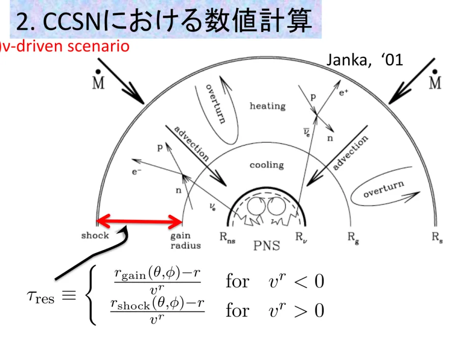
1)ν-­‐driven  scenario

Janka,    ‘01

Rstalled_shock~100km €

2.  CCSN における数値計算  

1)ν-­‐driven  scenario          (no-­‐explosion  under  spherical  symmetry)

€

13M_sun  Liebendorfer+,’01

2.  CCSN における数値計算  

Rshock(km)

Buras+,’06

2D

1D

Buras+,’06

Marek&Janka,’09

15M_sun

11.2M_sun

Takiwaki+,’11

13M_sun

Suwa+,’10

1)ν-­‐driven  scenario          (successful  explosions  in  mulC-­‐D)

2.  CCSN における数値計算  

1)ν-­‐driven  scenario

€

Janka,    ‘01

€

τ_heat ≡ −e_bind

Q ˙ Time  scale  of  binding  energy  to  be  0  (unbound)

– 22 –

Fig. 12.— Mean shock radii as a function of post-bounce time.

explosion (Janka 2001; Murphy & Burrows 2008). Here τ_res is the residency time scale defined by τ_res ≡

! _r

gain(θ,φ)−r

v^r for v^r < 0

r_shock(θ,φ)−r

v^r for v^r > 0 (43)

and represents how long a comoving fluid element in the gain region is expected to be exposed to the neutrino heating. Here we note both denominator and numerator are measured in the Eulerian frame. τ_heat is the heating time scale defined by

τ_heat ≡ −ε_bind

Q˙ (44)

where ε_bind and ˙Q ≡ e^6φαQ^µn_µ (see, Eq. 14) are the binding energy and the net heating rate of a fluid element, respectively. τ_heat represents how long it takes to get unbounded from the gravitational field for a fluid element. As for the definition of binding energy ε_bind, we adopted a Newtonian treatment expressed by

ε_bind ≡ ρ

"

u^tε + 1

2v_ivⁱ + φ_{N T}

#

(45) where φ_{N T} < 0 is evaluated by solving Eq.(27). Then the heating efficiency is derived by averaging each time scale τ_res and τ_heat and take their ratio. Here the averaging is performed for all numerical cells with ε_bind < 0 and ˙Q > 0. If τ_res is longer than τ_heat, a fluid element is From Fig. 13, we see both of 3D models are efficiently heated compared to 1D models. This is because the radial flows can be converted to the lateral flows in 3D which lengthen τ_res. Furthermore, on one hand,

2.  CCSN における数値計算  

1)ν-­‐driven  scenario          (successful  explosions  in  mulC-­‐D)

KT,Kotake,Takiwaki,’12

MulC-­‐D  effects  are  key  to  successful  explosion

2.  CCSN における数値計算  

2)magneto-­‐rotaConal  explosion  (MRE)

Takiwaki+,’08  (2D-­‐axisymmetry) Scheidegger+,’10  (3D)

Possible  amplificaCon  mechanisms  are            1)  winding  effect  

         2)  magneto  rotaConal  instability(MRI)

2.  CCSN における数値計算  

 Microphysics  

• EOS  of  baryonic  maiers  above  nuclear  density  (ρ>~2x10¹⁴g/cc)    

• Neutrino  transfer    (Burrows+  ’06,  Marek&Janka,’09,  Suwa+,’10,Takiwaki+,’11)  

 

一般相対論    

 

３次元の効果  

 

磁場の影響 

2.  CCSN における数値計算  

  BSSN  formalism      (metric)  

  RelaCvisCc  (M)HD                                            

  3D-­‐Nested  grid

  Neutrino  radiaCon  (gray  energy)   1)  cooling  (leakage)  

2)  heaCng  (truncated  (M1)  method)  

Features  of  our  code          (see,  KT,  Kotake  &  Takiwaki,  ApJ,  ’12)

Numerical  scheme  (code)  

KT  &  Umeda,’10  

Roswog&Liebendorfer’03,  Sekiguchi,’10

Thorne’81,  Shibata+’11

€

G

= 8 π ^T

≡ 8 π ( ^T

+ T

)

Hydrodynamic  equaCons  (10+3  variables)

Neutrino  RadiaCon  equaCons  (12xNene  variables) BSSN  equaCons  (17  variables)    +    Gauge  condiCons

Numerical  scheme  (code)  

Matsumoto,’07

Matsumoto,’07

To  obtain  conCnuous  “

∇

(1)  2D  interpolaCon

(2)  1D  interpolaCon

2)MRE

GW  emission  from  rotaCng  star  

1)ν-­‐driven  explosion

“Spherical”  explosion “Oriented”  explosion

But  there  are  several  problems…  

  Usually  CCSNe  occur  very  far  from  us!  

                         θ~(10

cm/10

cm)=10

  Explosion  occurs  deep  down  the  star!  

                         opCcally  thick

1000km

GW  emission  from  rotaCng  star  

Kotake,’11,  "GravitaConal  Waves  (from  detectors  to  astrophysics)"

Then,  how  can  we  decipher  which  mechanism   affects  mostly  on  the  explosion?

GW  emission  from  rotaCng  star  

As  candidates  of  strong  GW  emiiers mergers  of  compact  stars  

(NSNS,NSBH,BHBH)

Core  Collapse  Supernovae   (CCSNe)

occurrence  

frequency

Phinney+,’91 Mannucci+,’07

GW  Amp@src  

GW  emission  from  rotaCng  star  

     h=A_GW/D  ~10^-­‐24    (with  D=10Mpc)   (h/sqrt(100Hz)~10^-­‐25)  

Can  we  detect  such  extraordinary  small  signals?

h/sqrt(f)

GW  emission  from  rotaCng  star  

What  we  have  to  do  is  to  predict  

gravitaConal  waveforms  and  neutrino  luminosiCes   as  precisely  as  possible  in  advance.  

• Full  general  relaCvisCc  

• MulC-­‐energy  &  mulC  flavor  neutrino  radiaCon  

• 3-­‐D  

• (Magneto-­‐hydrodynamical)  

                 simulaCons  are  indispensable.

GW  emission  from  rotaCng  star  

Aim  

 By  using  full  3DGR-­‐Rad.  hyd.  code,  

     we  invesCgate  rotaConal  effects  on  GW  emission  

In  Oi+,’12,  the  computaConal   domain  is  only  one  quadrant.

In  Oi+,’07,  they  neglect  ν-­‐cooling

€

ϖ

= 1000 km

Progenitor:  15Msun  (WW95)  

EOS:  Shen  eos  (Shen+,’98)+e^-­‐e⁺+photon(+neutrino)   IniCal  rotaConal  profile

We  calculated  4  models  with  varying  Ω₀

€

Ω₀ = 0, π

6 , π

2 ,π^{(rad / s)} According  to  Hegar,  ’05,   Ω₀~1  (rad/s)  at  maximum.

Numerical  scheme  (iniCal  condiCon)  

 128³cells  *  9  Level  nested  structure      (dx_min~450m)  

 Random  perturbaCon  

（

）

 Cray  XT4  (512core)  @  NAOJ,          ~1.3ms/1day  

400km

0<T_pb<50ms

 If  CCSN  occurs  within  our  galaxy  (D<10kpc)  

     and  progenitor  rotates  sufficiently  fast  

（

）

 ObservaCon  along  polar  axis  also  gives  us  possibility  of  detecCon.  

Results  (GW  spectra)  

Results  (GW  spectra)  

Comparison  with  Oi+,’12

Spectral  peak  appears  at  similar  value  ~670Hz(ours)                                                                                                                                            ~700Hz(Oi+’12)

RotaConal  signatures  in  GW  spectra  

rotaConal  

axis equator

RotaCon

immediately     a2er  the  

bounce late  phase equator polar  axis

~700Hz ~200Hz

l=2  mode

Where  do  these  signals   come  from  ?

RotaConal  signatures  in  GW  spectra  

SpaCal  distribuCon  of  GW  source  toward  polar  axis

Ω=pi

where

GW  extracCon  by   quadrupole  formulae  

€

log ˙ ˙ I _xx² −I ˙ ˙ _yy²+( )2 ˙ ˙ I _xy ²

GW  emission  from  one-­‐armed  spiral  wave  

One-­‐armed  Spiral  wave  is  the  GW  (@~200  Hz)  emiier

Equatorial  plane

What  determines  emission  @~200Hz?

 

~

T_pb=

GW  emission  from  one-­‐armed  spiral  wave  

 50km                          100km                150km                                      (x²+y²)^1/2    km

€

Ω_aco + Ω_rot

€

Ω_rot

“F_peak-­‐100Hz”  reflects  rotaConal  Cme  scale  above  the  PNS(?)

 ~200Hz  is  determined  from  Doppler  shi‚  (rot.  +  sound  velocity)  

 Since  Ω_aco  (~100Hz)  is  hardly  changed  by  progenitor  rotaCon  

Conclusions  

① CombinaCon  of  low-­‐T/W  instability  and  spiral   SASI  can  leave  its  message  in  GW  emission.  

② Its  emission  frequency  can  be  determined   from  Doppler  shi‚.  

NAOJ

Usually  CCSNe  occur  far  from  us  and  it  is  very  difficult  to   resolve  angular  dependence  of  asymmetry.

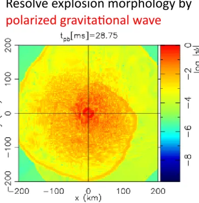
c.f.,  Tanaka+,’12 Resolve  explosion  morphology  by  

polarized  EM  wave  

9 per 2 ms, i.e., rotational period is Trot ∼ 8 ms. This rota-

tional time scale corresponds to 2/T_rot = 250 Hz, where numerator 2 in left hand side comes from 2 emissions of a polarized wave during one rotation. This value 250 Hz is consistent with the aforementioned gravitational wave frequency, F ∼ 200 Hz. Therefore, we claimed the strong narrow band emission, appeared after the neutronization phase in our most rapidly rotating model R0pi, obviously originated from the one-armed spiral wave.

FIG. 6. Localized gravitational wave source term ψ along the equatorial plane for model R0pi. As seen, one-armed spi- ral wave emit strong gravitational wave and the spiral wave rotates approximately 90^◦ per 2 ms.

To assess the origin of narrow band emission at F ∼ 200 Hz which is shifted ∼ 100 Hz higher compared to other models, we analyzed rotational-acoustic wave fre- quency. To do this, we defined following two rotational velocities Ω_aco and Ω_rot and plotted them in Fig. 7.

Ω_aco ≡ 2 C_s 2π!

x² + y² (47) Ω_rot ≡ 2 V_φ

2π!

x² + y² (48) In Fig. 7, spatial profiles of Ω_aco + Ω_rot (solid) and Ω_rot (dashed) along the x axis at different time slices are plot- ted.

FIG. 7. Spatial profiles of Ωaco+Ωrot (solid) and Ωrot (dashed) along the x axis at different time slices. Color represents post bounce time labeled by numbers appeared in the panel.

As seen in the figure, rotational-acoustic wave fre- quency (solid lines) shows Ω_aco +Ω_rot ∼ 250 Hz at 60 km

! R ! 120 km. This frequency is consistent with both narrow band emission above the protoneutron star seen in Fig. 5 and our former estimation using Fig. 6. Re- markably, Ω_rot is comparable to Ω_aco and Ω_rot amounts

∼ 100 Hz which is approximately the same value with peak shift seen in model R0pi during the prompt convec- tive phase. Therefore, we hope we can extract some infor- mation about rotation above the protoneutron star by es- timating gravitational wave’s peak shift. Here, however, we assume Ω_aco does not change significantly from model to model in highly convective region, i.e., the sound veloc- ity C_s does not depend so much on the initial condition at precollapse phase. We consider this assumption is quite reasonable because many previous studies with different initial conditions, such as magnetic field or progenitor mass, reported gravitational wave emission with peaking

∼ 100 Hz during prompt convective phase [1, 16, 20].

Finally, we plot characteristic wave strain h_char with sensitivity threshold of gravitational wave detectors for Initial LIGO [8], Advanced LIGO [26] and KAGRA [11], in Fig. 8. To draw this figure, h_char is evaluated by Eq. (45) but without Hann window, therefore our re- sults show spectra of total emitted gravitational energy.

Observation along the equatorial plane produces broad band energy spectra with exceeding noise threshold over frequency range 100 ! F ! 1000 Hz. Faster rotation raises the chance to detect gravitational waves and this is consistent with results of [54]. Their results and ours are quantitatively similar with spectral frequency peak- ing at F ∼ 700 Hz and maximum amplitude of wave strain h_char(h_char/√

F ) is ∼ 6 × 10⁻²¹(2 × 10⁻²²).

Observation from polar region produces narrow band spectra with 2 peaks. First peak seen at F ∼ 1000 Hz is emitted during the neutronization phase (t_pb ! 8) and is considered to be originated from the low-T /|W| insta- bility. In non- or slowly rotating models, thus, it cannot be seen this first strong peak. Second peak appears at F ∼ 100 Hz in non- to moderately rotating models and is mainly radiated during the prompt-convective phase in our short calculation time. This peak comes from time scale of acoustic wave mode. On the other hand, the sec- ond peak is shifted upward to F ∼ 200 Hz in rapidly ro- tating model. As already explained, this peak shift is due to the low-T /|W| instability and is determined by combi- nation of acoustic and rotational time scale. In terms of gravitational wave detection from polar region, the sec- ond peak achieves S/N " 10 irrespective of rotational profile and the first peak marginally reaches S/N ∼ 10 only in our most rapidly rotating model.

IV. SUMMARY AND DISCUSSIONS

In this paper, we derived the gravitational wave emis- sion from rotational collapse and bounce of a 15 M_" star in full general relativity. Since observation by the gravi-

Resolve  explosion  morphology  by   polarized  gravitaConal  wave  

lumpy  structure oriented  structure

Toward  future  analysis