IPSS Discussion Paper Series
National Institute of Population and Social Security Research Hibiya-Kokusai-Building 6F 2-2-3 Uchisaiwai-Cho
Chiyoda-ku Tokyo, Japan 100-0011 (No.2013-E01)
Child Support and the Poverty of Single-Mother Households in Japan
Akiko S. Oishi (Chiba University)
August 2013
IPSS Discussion Paper Series do not reflect the views of IPSS nor the Ministry of Health, Labor
and Welfare. All responsibilities for those
papers go to the author(s).
Child Support and the Poverty of Single-Mother Households in Japan
1Akiko S. Oishi
2Faculty of Law and Economics Chiba University
August 2013
Abstract
This paper estimates a noncustodial father’s ability to pay child support and measures the extent to which the introduction of a child support guideline would have on poverty and welfare benefits of single-mother households in Japan, taking into account possible feedback on the mother’s labor supply. It turns out that the father’s human capital and the pattern of spousal pairing significantly affect the father’s income. Policy simulation predicts that the introduction of the Wisconsin child guideline not only reduces the poverty rate of single-mother households, but also reduces the welfare cost associated with the provision of the Child Rearing Allowance. On the other hand, it is predicted that introducing the time limit to the CRA adversely affects the well-being of the single-mother households, and the decline in income is prominent in lower income quintiles.
1
The data used in this paper was made available by the Japan Institute of Labour Policy and Training. I would like to thank Yanfei Zhou, Chien-Chung Huang, Aya Abe, Yoshihiro Kaneko, and Lisa Karakas for their comments. This study is supported by the Japan Society for Promotion of Science Grant-in-Aid for Scientific Research (Grant Number B-23330100-5001 and C-23530269) and Grant-in-Aid for Scientific Research on Innovative Areas (Grant Number 21119004). Remaining errors are my own.
2
Corresponding author: Faculty of Law and Economics, Chiba University, Yayoi-cho 1-33, Inage-ku,
Chiba, 263-8522, Japan. Telephone: +81-43-290-3579. E-mail: [email protected].
1 Introduction
In many OECD countries, past decades have seen a notable increase in the number of children living in single-parent households. Japan is no exception. The number of
single-mother households in Japan has risen by 25% since 1998, reaching 1.23 million in 2011.
1As of 2010, 7.6% of children below the age of 18 were raised in single-mother households, including those who were living with grandparents and other relatives (Statistics Bureau, 2010).
The most significant feature of single-mother households in Japan is its poverty.
Fifty percent of lone-parent households in Japan in 2009 were poor, compared with 12.7%
of two-parent households, more than a four-fold difference (Ministry of Health, 2011).
Japan ranks the highest among the OECD countries with regard to the poverty rate of lone-parent families in the mid-2000s (OECD, 2009).
Developed countries, in general, have cash benefits for poor families with children.
In addition to these public cash transfers, many countries have established schemes to ensure private cash transfers, so-called “child support” or “child maintenance,” between the noncustodial and custodial parent (Skinner, 2007). For example, the Child Support Act was enacted in the UK and New Zealand in 1991. In the US, the history of child support dates back to 1975 when Congress created the Child Support Enforcement Program.
What motivated legislators in these countries to pass laws to establish child support enforcement were the expectations that stronger child support enforcement would not only improve children’s welfare but also reduce welfare costs and caseloads. Huang, Garfinkel, and Waldfogel (2004) have found that improvements in child support
enforcement during the period of 1980-1999 reduced welfare caseloads by 9% in 1999.
Neelakantan (2008) has estimated that higher child support payments led by changes in child support policy contributed to a decline in the percentage of divorced mothers on
1
Unless otherwise noted, statistics referred to in this paper are based on the Ministry of Health,
Labour and Welfare’s National Survey on Single-mother Households in 2011.
2 welfare.
In Japan, however, the government has not adopted any measures to ensure child support so far despite the growing fiscal pressure to cut welfare expenditure. In fact, the government has decided to lower Public Assistance benefits by 4-10% for the first time in 9 years in 2013. The Child Rearing Allowance (CRA), which is provided to a lone parent with children up to the age of 18, has also been reduced annually for years. Moreover, it is likely that the government might resume a time limit to the CRA, which was supposed to be put into effect in 2008 but was suspended due to a rise in the poverty rate.
Although past studies have shown that child support has had a sizable effect on reducing poverty of lone-parent households (Bartfeld (2000); Sorensen and Hill (2004);
Skinner (2007)), a number of studies report a greater potential of nonresident fathers’
ability to pay child support (Garfinkel and Oellerich (1989); Garfinkel, Oellerich, and Robins (1991); Bartfeld (2000)). In particular, Garfinkel et al. (1991) estimate that an introduction of a “perfect” system would reduce the poverty rate of lone-parent households eligible for child support from 38.9% to 31.7%. Huang (1999) estimates the introduction of the Wisconsin child-support guideline to Taiwan would halve the poverty rates of divorced- and separated-mother families.
A few studies, however, have taken into account the effects of child support on the labor supply of mothers. Economic theory predicts that an increase in one’s unearned
income would reduce one’s labor supply, assuming that leisure is a normal good.
2Thus, the mothers’ take-home pay will decrease if the amount of child support increases (Hu, 1999).
In this sense, prior research which ignores the behavioral responses of mothers to an increase in child support may have overestimated its effect on the poverty of single-mother
2
The economic theory also predicts that a person’s labor supply will change if his/her wage rate net of taxes decreases. For a noncustodial parent, child support enforcement proportional to one’s earnings translates into an increase in marginal tax rate, which lowers his/her wage rate. Work effort of the noncustodial parent will increase if the income effect associated with lower wage rate
dominates the substitution effect, and vice versa.
3 households.
The purpose of this paper is to estimate a noncustodial father’s ability to pay child support and to measure the extent to which the introduction of a child-support guideline would have on poverty and welfare costs of single-mother households, taking into account possible feedback on the mother’s labor supply. No research has been conducted that
estimates the effect of child support on the well-being of single-mother households in Japan.
This study also departs from the existing literature on child support in that it focuses on the distributional aspect of the reform, including the estimation of income distribution.
The main contributions of this paper are as follows. First, I estimate the fathers’
ability to pay child support using nationally representative data on child-rearing households that includes information on noncustodial fathers. It turns out that the father’s human capital and the pattern of spousal pairing significantly affect the father’s income. I also estimate a model of the mothers’ labor supply function to capture their responses induced by the reforms in child support and the CRA.
Second, I simulate the introduction of the time limit to the CRA and examine its distributional and fiscal effects, taking into consideration the mothers’ behavioral responses.
To assess the well-being of single-mother households, two criteria are used: the first
criterion is the poverty rate, i.e., the proportion of households living below the poverty line, which is set at 50% of the median income of child-rearing households in 2010. Another criterion is the proportion of households whose income falls below the minimum cost of living (MCL) defined by the Public Assistance system. The MCL is one of the
constitutional rights, and the amount of the MCL is calculated taking into account the
family structure, age, and place of residence. Simulation results show that the introduction
of the time limit raises the proportion of poor single-mother households in terms of both
criteria for poverty. While the time limit is effective in reducing public spending of the
CRA, a large amount of the reduction comes at the expense of the well-being of households
in lower-income quintiles.
4
Third, a policy simulation on introducing the Wisconsin child-support guideline is conducted. This simulation is important because in Japan, where there are no official child-support guidelines, no estimate has been made to assess the potential gains of establishing and enforcing the child-support guidelines. The simulation results show significant improvements in poverty rates of single-mother households, which is
accompanied by a reduction of welfare costs. Specifically, a majority of the cut in welfare costs comes from the upper-income quintiles.
The first section below presents an overview of the economic situation of
single-mother households in Japan and the government’s policies towards them. The second section describes the data used in the empirical analysis. The third section explains the methodology of policy simulation. The fourth section shows regression results. The fifth section presents simulation results. The sixth section concludes.
1. Policies Related to Single-Mother Households
This section describes the definition of single-mother households and explains policies that affect their well-being.
Definition of a Single-Mother Household
In this paper, a single-mother household is defined as a household where a mother is raising
her children, who are unmarried and below the age of 18, without a father. This definition
includes households in which a single mother and her children are living with her parents or
other relatives. Among 1.54 million children being raised in single-mother households, 433
thousand (or 28%) live with their grandparents or other relatives, which far exceeds the rate
of co-residence prevalent among households with children (17.2%) (Statistics Bureau,
2010). A single mother could be either never-married, widowed, or divorced, but it should
be noted that, unlike in the US and EU countries, 81% of single mothers result from
5
divorce.
3Japan’s Family Law stands out from other advanced countries in that a couple with children can file for divorce with neither judicial procedure nor legal arrangement of child support. Moreover, there is no law which assures the child’s right to receive economic support from their noncustodial parent. As a result, mothers who are in the process of divorce tend to give up negotiating the arrangements of child support and distribution of property with their husbands in exchange for the custody of their child.
Child Rearing Allowance
Child Rearing Allowance, whose beneficiaries have reached 1.07 million (including 61 thousand single-father households) in 2012, is a means-tested transfer provided to
lone-parent households living with a child/children up to the age of 18. The benefit amount decreases proportionally to the sum of a mother’s earnings and 80% of child support. For example, a mother who makes less than 1.30 million yen a year and lives with one child can receive a “full benefit” of 41,480 yen a month (≓0.5 million yen per year). If she makes between 1.30 million and 3.65 million yen a year, she can receive a “partial benefit,”
the amount of which varies between 9,720 to 41,170 yen, according to her income. A mother is no longer eligible for the CRA if she makes more than 3.65 million yen a year. An additional benefit of 5,000 yen a month is provided if there are two children up to the age of 18 in the household, and 3,000 yen for each additional child thereafter. As of March 2012, 57.4% of CRA beneficiaries receive “full benefit” and 42.6% receive “partial benefit”.
Faced with a rapid increase in the number of CRA beneficiaries and the worsening of financial conditions since the collapse of the “bubble” economy in the 1990s, the
government has been lowering the income ceiling for receiving the CRA as well as the amount of benefits. One of the major reforms in the CRA took place in 2002 when the income ceiling for receiving the “full benefit” was reduced from 2.04 million yen to 1.30
3
Out-of-wedlock birthrate is very low, with 2.15% of total births in 2010.
6
million yen, resulting in a decline in the number of “full benefit” recipients by 119,000, or 18.5%. In the 2002 reform, the government introduced a time limit of five years to the CRA by which the amount of benefits provided to single-mother households can be reduced to a half after their fifth year. Those households with children below the age of eight are exempt from the time limit. This measure had been scheduled to be put into effect in April 2008 (five years after the reform) but was suspended due to a rise in the poverty rate.
Policies towards single-mother households in Japan share common features of the Welfare Reform in the US, which emphasizes self-sufficiency through their employment (“Work First”). The fact is that 80.6% of single mothers are employed, and many of them work 2,000 hours a year (Oishi, 2013).
4Although more than half of single-mother
households are in poverty, 110,000, or 8.8% of them, were on welfare in 2011. Despite their attachment to paid labor, their median earned income in 2011 barely reached 1.5 million yen, for job opportunities for women are limited in the Japanese labor market, and about half of single mothers work on a non-regular basis and earn low wages.
5Under these circumstances, empirical studies in Japan have found little evidence to support resuming the time limit. Oishi (2012a) reports that, for single-mother households, the risk of poverty doesn’t decline with the years after divorce. Zhou (2012)finds no significant difference in the degree of economic self-sufficiency between a group of single mothers who have been divorced less than five years and a group of those who have been divorced more than five years.
Child Allowance
In addition to the CRA, Child Allowance (CA) is provided to households with children.
Since 2009, when the Democratic Party came into power, CA has undergone drastic
4
The employment rate of single mothers fell from 84.5% in 2006 to 80.6% in 2011, but it should be noted that the 2011 Survey was conducted seven months after the Great Quake and the accident of the Fukushima Dai-ichi nuclear plant.
5
Y. Abe (2011) describes the characteristics of the female labor supply in Japan.
7
changes. Until March 2010, CA had been a means-tested benefit which provided 5,000 yen a month to each child up to the age of 18. The benefit was raised to 10,000 yen a month if the child was below the age of three. If there were more than two children in the household, 10,000 yen a month was provided to each additional child. The income ceiling for receiving CA for a household with a child and a spouse who earned less than 1.30 million yen a year had been 6.08 million yen. Beginning in April 2010, a universal CA of 13,000 yen a month had been paid to every child below the age of 16. This universal CA, called “Kodomo-teate”
in Japanese, lasted only two years and was replaced by a new, means-tested CA in April 2012. Currently, 10,000 yen a month is paid to each child below the age of 16 and the benefit is raised to 15,000 yen a month if the child is below the age of three. If there are more than two children in the household, 15,000 yen a month is provided to each additional child. The income ceiling was set at a higher level than the old CA, with 9.12 million yen for a household with a child and a spouse whose annual income does not exceed 1.30 million yen.
Public Assistance
Public Assistance (PA), often referred to as the “last resort safety net” in Japan, is provided upon receipt of an application from a household in need and after a careful examination of the application. First, the examination is accompanied by vigorous means and asset tests, as well as proof of non-support from one’s family members, who not only include parents and children but also siblings, aunts, and uncles. In the case of a single mother, her application cannot be accepted unless she provides enough evidence of non-support from her
ex-husband (the child’s father). Second, holdings of financial assets as well as real estate and houses are not allowed, and they must be sold preceding the application for PA. Third, the person will not be able to receive assistance if he/she is judged as capable of working.
Past studies on poverty in Japan have estimated the PA take-up rate (defined as the
percentage of those who actually are beneficiaries of the program among all those who are
8
eligible) to be low, varying between 4% to 40% depending on the region and the time of the study (A. K. Abe (2003); Komamura (2007); Tachibanaki and Urakawa (2006)).
The amount of PA is calculated by subtracting the household’s final income (including benefits from other welfare programs such as public pension, CA, and CRA) from the MCL. The calculation of the MCL takes into consideration the differences in living costs among different regions of the country, family structure, and household members’ age (NIPSS, 2011). For example, the MCL for a single mother with a 4-year-old child is 189 thousand yen a month if she lives in a large city and 132 thousand yen a month if she lives in a rural area. An additional benefit for single-mother households and elderly households had once been abolished in April 2007; however, the benefit for single-mother households was revived in December 2009 after the Democratic Party came to power.
6As of July 2012, 1.56 million households or 2.13 million persons (1.67% of the population) received some type of PA. The proportion of welfare recipients to the population is smaller for Japan as compared to other OECD countries. Single-mother households comprise 7.4% of PA recipient households, while elderly households make up the largest share (43.5%). Although the number of single-mother households receiving PA has been increasing, its share in the total has dropped by one percentage point in the last decade.
Child-Support Guidelines
Unlike in other developed countries, the Japanese government has not established any official guidelines to assure child support from a noncustodial parent. As a result, only 19.7% of divorced mothers were receiving child support in 2011 (Ministry of Health, Labour and Welfare, 2011). To improve the situation, the government has been encouraging
6
Schaede and Nemoto (2006) have found that historical variations in PA spending and welfare
coverage rates are significantly affected by the number of seats held by the Liberal Democratic
Party and concluded that politics matter more than socioeconomic factors in Japan.
9
divorcing parents to adopt a child-support guideline proposed by a study group of lawyers in Tokyo and Osaka. This guideline, called yoikuhi santei hyo in Japanese, was first published in an academic journal in 2003 and is increasingly referred to in divorce cases and private negotiations for an amicable divorce. The Japan Federation of Bar Associations, however, has issued a statement criticizing that the guideline acknowledges a broad
expenses deductible from the noncustodial parent’s income, thereby making the amount of child support too low. For example, depending on the earnings of the custodial parent, the guideline sets the amount of child support between 4.8% and 12% of the gross income of a noncustodial parent who has one child younger than the age of 15. These percentages are lower than those of other developed countries where the proportion of child support to national average earnings varies between 8.0% to 18.3% (Skinner & Davidson, 2009).
In the US, each state has established child-support guidelines that take into account three factors: father’s income, mother’s income, and the age and number of children.
According to the Massachusetts guideline, child support is basically determined proportionally to the noncustodial parent’s income and the child’s age. Percentages are higher when the incomes are higher and when the child is older. States like Indiana and Kansas adopted an income-sharing model, in which percentages decline as the combined income increases. In Kansas, the percentages are higher when the child is older, while in Indiana the percentages do not vary according to the child’s age (Bartfeld, 2000).
Each guideline has its merits and demerits. First, other things being equal, the risk of noncompliance should be lower in Massachusetts because the percentage for the
low-income noncustodial parent is set at lower levels than those in Kansas and Indiana.
Past studies have found that child-support noncompliance is more prevalent among poorer noncustodial parents (Phillips and Garfinkel (1993); Zhou (2012)) . Second, as in
Massachusetts, setting the percentage of child support progressively to income would not
10
only reduce labor supply but also result in income bunching of the noncustodial parent.
7Since the percentage rises with the income brackets, the budget set of the noncustodial parent draws a piecewise linear line with kinks at each point where the marginal child support rate jumps. In such circumstances, individuals tend to concentrate their earnings at certain levels (“income bunching”) (Saez, 2010). Third, setting higher percentages for older children may result in less work effort of the noncustodial parents at certain periods of their lives because they can easily foresee the timing of the increase in their child-support payments.
In the simulations that follow, I adopt the simplified version of the Wisconsin child-support guideline described in Bartfeld (2000). Since the Wisconsin guideline sets the percentage constant irrespective of the incomes of both noncustodial and custodial parents, we can omit the behavioral responses of the noncustodial parent caused by kinks in the budget line. The percentage varies only with the number of children irrespective of their ages (17% for one child, 25% for two children, 29% for three children, 31% for four children, and 34% for five children).
2. Data
The data used in the analysis was drawn from “A Survey on Child Rearing Households”
(SCRH), which was conducted in November 2011 by the Japan Institute for Labour Policy and Training, a research arm of the Ministry of Health, Labour and Welfare. The SCRH surveys a randomly selected sample of 4,000 households (2,000 two-parent households and 2,000 lone-parent households) with children below the age of 18 chosen from the
Residential Registry throughout Japan. In order to have enough numbers of lone-parent households, the sampling was conducted separately for two-parent households and lone-parent households (including single-father households). As a result, data on 1,435
7
Past studies have found little evidence that child support reduces labor supply of the noncustodial
parents (Klawitter (1994); Freeman and Waldfogel (2001)).
11
two-parent households (response rate = 71.7%) and 783 lone-parent households (response rate = 39.1%) was collected. Data on lone-parent households consists of 699 single-mother households and 84 single-father households.
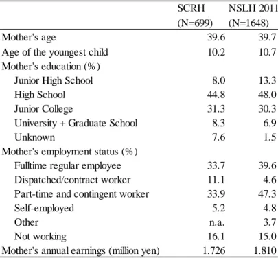
Although the response rate for lone-parent households is low, socioeconomic attributes of the respondents with respect to age, education, occupation, income, and the age of the youngest child are similar to those of the 2011 National Survey on Lone-parent Households, the most comprehensive survey on lone-parent households conducted by MHLW every five years (Table 1).
I believe that the SCRH is one of the best surveys available for the analysis on single-mother households and child support in Japan. First, due to their low incidence and underreporting, most of the existing surveys fail to have ample number of single-mother households for analysis. For example, the National Survey on Family Income and Expenditure, one of the largest household surveys and whose sample size amounts to 52,000 households, reported only 629 single-mother households in the sample in 2009.
Second, information on noncustodial parents is hardly attainable. Even the National Survey on Lone-parent Households, which has 1,648 single-mother households in its sample, lacks information on nonresident fathers. Third, information on PA is also unattainable in most surveys, since people used to believe that some form of social stigma is attached to PA.
The SCRH collects information on a noncustodial father’s education and income at the time of divorce, which allows us to estimate the father’s ability to pay child support. In addition, the SCRH asks the respondent whether the household is receiving PA or not, which allows us to estimate how the proportion of welfare recipients would change if reforms were put into effect.
I confine the sample to respondents who are: i) divorced mothers, and ii) have
necessary information for policy simulation. Thus, the sample for the policy simulation
comprises 498 single-mother households. I also use a sample of two-parent households to
compare the income distribution with that of single-mother households.
12 3. Method
Estimating the Father’s Current Income and Child Support
To simulate the effects of the introduction of the child-support scheme on the poverty of single-mother households, we need to know the father’s current income. In most cases, however, such data are unavailable and attempts to estimate the father’s income have been made.
Using the Survey of Income and Program Participation (SIPP), Sorensen (1997) estimates the nonresident fathers’ ability to pay child support in total by reweighting the income data for nonresident fathers who can be identified in the SIPP sample. Reweighting is needed because nonresident fathers are, in general, underrepresented in surveys.
8Her method cannot be applied here because our question is not the total amount of child support that could be paid by nonresident fathers as a whole but the amount of child support that could be received by each single-mother household.
Garfinkel and Oellerich (1989)and Huang (1999)estimate the income of
noncustodial fathers using the attributes of mothers. Specifically, they use income data for a sample of married men with children and regress it to the wives’ socioeconomic attributes.
Then, they impute the nonresident father’s income for each single-mother household using the mother’s attributes. A major problem inherent in this method is how to deal with the difference in income between married and divorced men, for existing studies report that divorced men earn less than their married counterparts(Sorensen (1997); Oishi (2012b)).
Estimating the model by Heckman’s two-step method could be a solution, but Garfinkel and Oellerich (1989) fail to adopt Heckman’s procedure because the estimated Mills’ ratio (selection term) was negative and insignificant. Were they successful, Heckman’s procedure is not enough to cope with the fact that a significant proportion of divorced men remarry.
8
Sorensen (1997) reports that the number of single-mothers in the SIPP outnumbers that of the
nonresident fathers by 15%.
13
Oishi (2012b)has reported that remarried fathers share similar socioeconomic features as married, never-divorced fathers, and their earnings are higher than those of divorced fathers who stay single after divorce. Assuming that socioeconomic attributes (including marital status) of the nonresident father are the same as those of the single mother may lead to an underestimate of the father’s income.
One of the features of the SCRH is that it collects information on education and annual income of the noncustodial father. Unfortunately, 78 out of 498 divorced mothers did not report the noncustodial father’s income. Thus, using a sample of 420 single-mother households, I impute the noncustodial father’s income for each household by regressing the father’s income to a vector of variables, including the father’s education and the mother’s socioeconomic attributes. It should be noted that the father’s income is reported as a categorical variable, and at the time of divorce. Therefore, I take the middle value of the income bracket and convert it to 2010 prices so that it could be used in the regression. In addition, I include a variable indicating the length after divorce as an explanatory variable to account for the father’s wage growth after divorce.
Taking into account the number of children in the household, child support for each household is estimated by applying the Wisconsin guideline to the father’s income.
Estimating the Child Rearing Allowance and the Child Allowance
As described in section 2, CRA is primarily determined by the mother’s earned income, child support, and the number of children. Estimation of the CRA involves three steps. The first step is to calculate the mother’s taxable income (E
n) which is given by
0.8 ∙
where E
gis the mother’s gross earnings, D
sis tax deduction for salaried workers, D
ssis tax
deduction for social security contributions, and CS represents child support. The Japanese
14
tax system sets the minimum value of D
sat 650,000 yen for salaried workers. Since the amount of D
sgradually increases with the worker’s earnings, I calculated each mother’s D
sby applying the income tax schedule to the mother’s earnings. With regard to D
ss, the government has fixed its amount at 80,000 yen for all individuals who apply for the CRA.
Starting in 2002, 80% of child support from a noncustodial parent has been taken into consideration when deciding the amount of the CRA.
The second step is to calculate the income ceiling for receiving a “full benefit”
(C
full) and a “partial benefit” (C
part) for each household, which are given by
190000 380000 ∙ 100000 ∙ 150000 ∙ 1730000
where N is the number of dependent household members (including children), N
oldis the number of dependents aged 70 years old or older, and N
youngis the number of dependents between the age of 16 and 22.
As the third step, the monthly CRA is calculated following the scheme below (note that the “full benefit” in 2010 was 41,720 yen a month).
CRA 41720 5000 ∙ 3000 ∙ ∙ 2 if
CRA 41720 ∙ 0.0182890 5000 ∙ 3000 ∙ ∙
2 if
CRA 0 if .
D
kid2is a dummy variable which equals one if there is more than one child who is eligible
for the CRA in the household, and zero otherwise. D
kid3is also a dummy variable indicating
that there are more than two children who are eligible for the CRA in the household. N
kidis
a total of the number of eligible children in the household.
15
Thus, a single mother of a young child who is not receiving child support can receive a full benefit unless her gross earnings exceed 1.30 million yen a year (C
full=570000, E
n=1300000 - 80000 - 650000 =570000 ). Even if her earnings exceed 1.30 million yen, she can receive a partial benefit if she makes less than 3.65 million yen a year (
1730000 570000 2300000, 3650000 80000 1270000 2300000).
Calculating Child Allowance is straightforward as it doesn’t vary according to the income of the household head (the primary earner). I assume that, for single-mother
households, the mother is the household head. Until March 2010, there had been an income ceiling for receiving CA. Thus, I calculate the amount of CA for the period of
January-March 2010 using the information on the number and age of the children in cases where the mother’s income did not exceed the income ceiling. Among the sample of single-mother households, very few were ineligible for CA in 2010 as the income ceiling had been set at a much higher level than that of the CRA. For the period of April-December 2010 when Kodomo-teate, a universal CA, had been provided, I calculate its amount using the information on the number and the age of the children.
Defining the Poor
In this paper, I define the poor in two ways. The first criterion is to define the poor as those who belong to a household where its equivalized income is below the poverty line. Since the focus of the study is poverty among households with children, I set the poverty line at 50% of the median equivalized income of child-rearing households using MHLW’s
Comprehensive Survey of Living Conditions 2010. Note that the median equivalized income
is calculated by dividing the median before-tax income of households with children by the
square root of the average number of household members 6.07 ⁄ √4.2 ∙
0.5 1.485 . Use of disposable income is common and preferred in poverty
research, but not being able to calculate the disposable income of the households from the
16 SCRH obliged us to use before-tax income.
9The second criterion is to define the poor as those who belong to a household whose income is below the MCL. The MCL varies with family structure, age of the household members, and the place of residence in particular to adjust for the differences in living costs (including housing). I calculate each household’s MCL using the information on individual and family attributes obtained from the SCRH. To make the poverty criterion consistent across different types of families, the MCL is calculated assuming that every household, either a single-mother household or a two-parent household, is a nuclear family (a family consisting of a parent/parents and a child/children). Then, the household is categorized as poor if the income of the parent(s) falls below the MCL.
Estimating the Behavioral Response from the Mother
As child support is unearned income for a single mother, its increase/decrease will reduce/increase the mother’s work effort through the income effect (Beller and Graham (1988); Garfinkel, Robins, Wong, and Meyer (1990); Hu (1999) ). In other words, the effect of introducing either the time limit or Wisconsin guideline on poverty could partly be offset by the change in the mother’s working hours. Taking such effects into consideration, I estimate the mothers’ labor supply function that can be expressed as:
∙ ∙
where H is hours worked by the mother, w is her wage rate, X is a vector of personal attributes, V is the unearned income, and ε is an error term. Child support from nonresident father and government transfers such as the CRA and CA are included in V.
This specification may not be appropriate if the amount of child support is endogenous (Hu, 1999). It is likely that unobservable factors affect both the child-support payment and the mother’s labor supply. One way to cope with the endogeneity problem is to estimate the
9
The SCRH does not have information on social security contributions, which are indispensable in
calculating the household’s disposable income.
17
model using instrumental variables (IV) for child support. Unfortunately, the amount of child support is, in most cases, missing in the SCRH, which prevents us from estimating the first-stage IV. As a result, I estimate the above model assuming that an increase in child support has the same effect on the mother’s labor supply as V. Using the estimated and her wage rate, the mother’s feedback to the policy change is calculated.
4. Descriptive Statistics and Regression Results Descriptive Statistics and the Incidence of Poverty
Table 2 presents descriptive statistics of the divorced single-mother households as
compared to two-parent households. On average, single mothers have a lower educational attainment than their married counterparts, with 6.6% of them graduating from universities.
They have fewer children and the proportion of mothers with preschool children is lower for single-mother households. Single mothers are more likely to work as regular employees, and their average working hours amounts to 1,854 hours a year, which is 18% longer than their married counterparts. Another notable feature is the type of residence. While 57% of two-parent households live in their own house, the respective figure for single-mother households is as low as 12.4%. On the other hand, 35% of single mothers live in their parents’ houses.
Table 3 compares the incidence of poverty between single-mother households and two-parent households, using different definitions of poverty. First, the incidence of PA is distinct among single-mother households, although the proportion (4.8%) of PA recipients in the sample of single mothers is lower than that of the official figure of 8.8%. The
proportion of households living below the MCL is estimated to be 38.0% for single-mother households and 11.4% for two-parent households, respectively. Using data from the
National Survey on Family Income and Expenditure, Tachibanaki and Urakawa (2006)
estimated the proportion of single-mother households living below the MCL to be 33% for
mothers with one child and 61% for mothers with two or more children. The take-up rate
(the ratio of households actually receiving PA to the number of households whose income
18
falls below the MCL) for single-mother households calculated from Table 3 is 12.6%, which is somewhat lower than the estimates from previous studies.
10If we use the poverty line of 1.485 million yen to define the poor, 58.9% of single-mother households are in poverty as compared to 17.6% of the two-parent households.
11Either of the two definitions of the poor exhibits a higher risk of poverty among single-mother households, especially households in which the mother is younger.
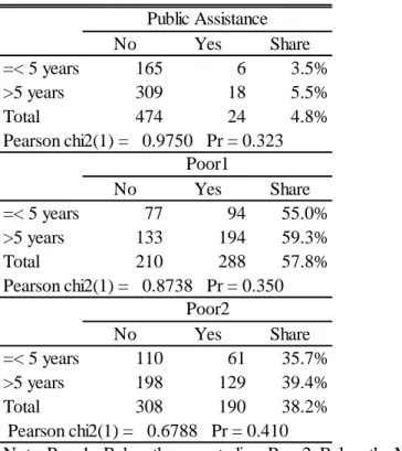
Table 4 examines if there are significant differences in poverty rates with respect to the years after divorce. In any of the poverty measures, no statistically significant differences are observed for those mothers who have been divorced for more than five years and those who have not. Although a more thorough examination should be conducted using panel data, these results question the validity of the time limit of five years in the CRA system.
Father’s income
The regression result for the fathers’ income is presented in Table 5. The father’s human capital and its interaction terms are significantly correlated with his income.
University-educated fathers earn much more than their high-school educated counterparts, and the effect is stronger if they were married to university-educated women. On the other hand, fathers who are not university-educated earn more if they were married to women who had worked as regular employees after graduating from school. The length after divorce is negatively associated with the father’s income, while the coefficient on its square is positive and significant. This means that the father’s income is lower if the divorce took place a long time ago, but the negative effect of the length after divorce on the father’s
10
Komamura (2007) estimates the take-up rate to be 18.5% in 1999. Tachibanaki and Urakawa (2006) estimate the take-up rate to be 16.3% in 2001.
11
These figures are higher than the officially reported poverty rates (50.8% for lone-parent
households and 12.7% for two-parent households) that are calculated based on equivalized
disposable income.
19
income gradually diminishes with years. The mother’s current age, which is a proxy for the father’s current age, is highly significant, and its effect becomes larger as the mother gets older. This phenomenon is known as “age-wage profile” commonly observed among Japanese male regular workers. The father’s income is higher by 0.65 million yen if he is paying child support.
Behavioral Response from the Mother
Table 6 reports the estimation result of the mother’s labor supply function. The wage elasticity is negative and significant. While age and education are insignificant, the
mother’s working hours are significantly longer if she is a regular employee and has a long job tenure. The coefficient of our interest, the effect of non-labor income on the mother’s labor supply, is negative and significant, suggesting that a 10% change in non-labor income of a single-mother’s household will cause a 1.2% change in the mother’s working hours.
5. Policy Simulations Time Limit
In this section I conduct two simulations to examine how changes in the CRA and child-support scheme affect poverty rates and welfare costs of single-mother households.
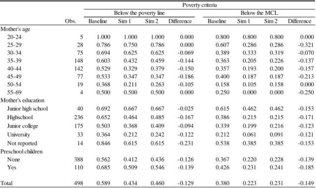
First, I explore the consequence of the introducing a time limit to the CRA. Specifically, I calculate the amount of the CRA that would be provided to single mothers if the benefit for those recipients who have been receiving the CRA for more than five years were cut to a half of its present amount. For simplicity, I assume the mother’s CRA spell is equal to the years after divorce.
Figure 1 shows the shift in the distribution of equivalized household income of
single-mother households caused by the introduction of a time limit to the CRA. For the
sake of comparison, the income distribution of two-parent households is also illustrated in
the figure. Due to the introduction of the time limit, the income distribution of the
20
single-mother households will slightly move to the left. The mothers’ behavioral response to the reduction in the CRA is barely visible, because about 60% of divorced single mothers are not subject to the reform either due to the presence of children below the age of eight or due to the short spell of CRA recipiency. As a result, the poverty rate as defined by the proportion of households below the poverty line will rise by 1.4 percentage-points, from 58.9% to 60.3% if the mothers’ behavioral response is taken into consideration (Table 7, Panel A). A rise in the poverty rate is more pronounced if the mother is older because these households are more likely to be receiving CRA for more than five years. The mothers’
increased work efforts induced by the change in CRA have little moderating effect on their poverty. Use of the alternative definition of poverty provides us with the same picture. The proportion of households whose income falls below the MCL will rise by 2.7
percentage-points, from 38.0% to 40.7%. It is not clear how many of them will actually become PA recipients, for being poor itself is insufficient to qualify for PA in Japan. Still, it is likely that an increase in poor households will have some effect on the number of PA recipients. If we assume that the PA take-up rate of single-mother households remains constant at 12.6%, a 2.7 percentage-point rise in the proportion of households whose income falls below the MCL will result in a 0.34 percentage-point increase in the proportion of PA recipients among divorced single mothers.
Although the simulated changes in poverty rates are modest, if we focus on those households that will be affected by the time limit, a significant rise in poverty will be observed (Table 7, Panel B). The proportion of households whose income is below the poverty line will rise by 3.7 percentage-points, from 67.7% to 71.4%. The rise in the proportion of households whose income falls below the MCL will be more distinct, a 6.9 percentage-point increase from 42.3% to 49.2%. As a result, the average household income (including CA, CRA, and other transfers) of the affected households will decline from 2.11 million yen to 1.93 million yen.
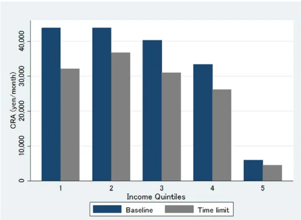
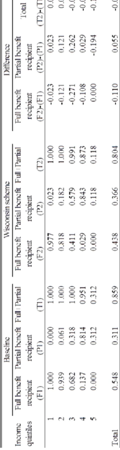
Figure 2 shows the change in per capita CRA (including non-recipients) by
21
quintile of the equivalized household income. The largest reduction in CRA comes from the lowest quintile where all households are receiving the “full benefit” due to their low income.
On the other hand, the change in the CRA in the highest quintile is minimal, because many of them are either non-recipients or receiving a small amount of money as the “partial benefit”.
The simulation predicts that the average amount of the CRA provided to
divorced-single-mother households will decline by 22%, from 33,676 yen/month to 26,329 yen/month. Thus, the introduction of the time limit will have a sizable impact on the financing of the CRA.
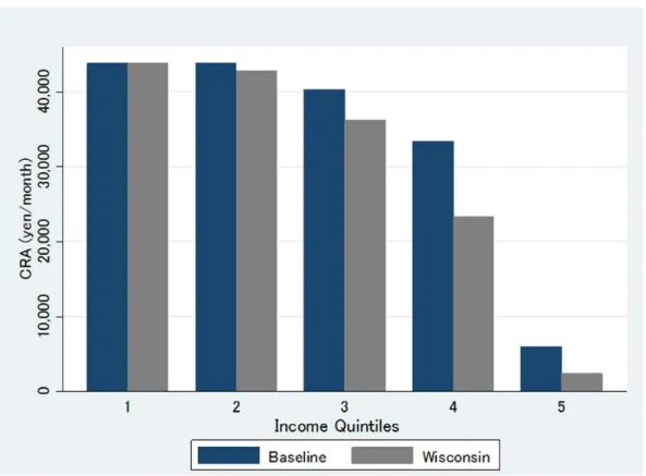
Introduction of the Wisconsin Child-support Guideline
Next, we examine the effects of the introduction of the Wisconsin child-support guideline.
It should be noted that this simulation illustrates the maximum potential which will be achieved by the introduction of the Wisconsin guideline, as 100% compliance is assumed.
Even in the US, the actual compliance rate falls far below 100%, so we have no reason to believe 100% compliance will be achieved in Japan. Nevertheless, it will be worthwhile for us to know the potential of the child-support scheme and consider it as a policy option.
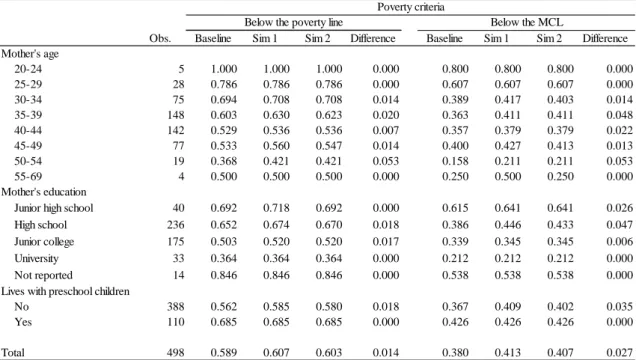
As is shown in Figure 3, the income distribution of single-mother households clearly shifts to the right if the Wisconsin guideline were introduced. The peak of the distribution moves very close to the poverty line, indicating that a middle mass of single mothers will be able to get out of poverty. As a result, the proportion of households below the poverty line drops sharply, from 58.9% to 46.0% (Table 8). If it were not for the decline in the mothers’ earnings caused by the mothers’ reduced work effort, the poverty rate will fall to 43.4%.
The proportion of households whose income falls below the MCL will decrease
from 38.0% to 23.1% if the adverse effect of mother’s behavioral responses were taken into
account. As we did in the simulation on the time limit, if we assume the PA take-up rate
22
remains constant, a 14.9 percentage-point drop in the poor households will lower the proportion of PA recipients among divorced single-mother households by 1.9
percentage-points.
Table 8 also shows the change in the poverty rate by the mother’s attributes, using the two definitions of poverty. First, the reduction in poverty is more prominent for those households with mothers in their late 30s and 40s. This is because the father’s income is higher if he is older. Second, mothers with a high-school education will gain most from the introduction of the Wisconsin scheme. Third, households with preschool children
experience a larger decline in poverty rate as measured by the MCL than their counterparts with no preschool children.
Comparing the two poverty criteria provides us with interesting features of the reform. In contrast to the case of the time limit where the two poverty rates move synchronously, the introduction of the Wisconsin scheme affects each poverty criterion differently. If we focus on households with mothers in their late 20s, the Wisconsin scheme reduces their poverty rate as measured by the MCL by 32.1 percentage-points, while the poverty rate as measured by the poverty line does not change. This continues to be the case in examining the changes in the poverty rates for households with mothers with a
junior-high-school education. These two groups of mothers more or less overlap due to the fact that those women who got married very young and divorced with children are more likely to be less educated.
12So are their ex-husbands, as assortative mating is a distinctive feature of marriage in Japan, with husbands and wives most likely to have the same level of education (Becker (1981); Raymo and Iwasawa (2008)).
13In such cases, child support is effective in helping the household to exceed the MCL, but not effective enough to exceed the poverty line, because less-educated fathers earn low wages, thereby resulting in a small
12
Note that, in Japan, the average age of first marriage for women was 28.8 years old and the average age of the first childbearing was 29.26 years old in 2010.
13