A structural analysis of the U.S. financial economy

A structural analysis of the U.S. financial economy

著者 Tsujimura Masako, Tsujimura Kazusuke

権利 Copyrights 日本貿易振興機構（ジェトロ）アジア

経済研究所 / Institute of Developing

Economies, Japan External Trade Organization (IDE‑JETRO) http://www.ide.go.jp

journal or

publication title

IDE Discussion Paper

volume 749

year 2019‑03

URL http://hdl.handle.net/2344/00050808

INSTITUTE OF DEVELOPING ECONOMIES

IDE Discussion Papers are preliminary materials circulated to stimulate discussions and critical comments

Keywords: flow-of-funds accounts; asset-liability matrices; financial net worth;

triangulation; dispersion indices JEL classification: C67, E44, O11

a

Rissho University, Tokyo, Japan; e-mail: tsujimura@ris.ac.jp

b

Keio University, Tokyo, Japan

IDE DISCUSSION PAPER No. 749

A Structural Analysis of the U.S.

Financial Economy

Masako Tsujimura ^a and Kazusuke Tsujimura ^b

March 2019

Abstract

The Flow-of-Funds Accounts of the Unites States have been published on a quarterly basis since 1945 up to the present time. In this paper, we will construct

‘sector × sector’ Stone and Klein-formula asset-liability matrices fully exploiting the huge accumulation of data. It allows us to trace the changes in the roles of the institutional sectors over the

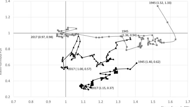
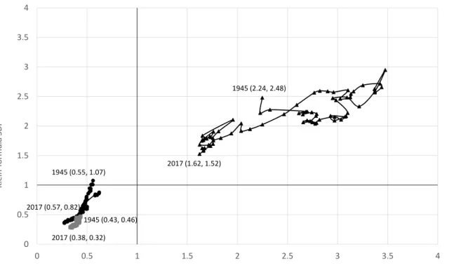
years by application of useful input-output analytical tools, such as triangulation

and dispersion indices. Although there is not too much change in the characteristics

of non- financial sectors, the roles of financial institutions have been changing as the

financial market develops and the deregulation advances.

The Institute of Developing Economies (IDE) is a semigovernmental, nonpartisan, nonprofit research institute, founded in 1958. The Institute merged with the Japan External Trade Organization (JETRO) on July 1, 1998.

The Institute conducts basic and comprehensive studies on economic and related affairs in all developing countries and regions, including Asia, the Middle East, Africa, Latin America, Oceania, and Eastern Europe.

The views expressed in this publication are those of the author(s). Publication does not imply endorsement by the Institute of Developing Economies of any of the views expressed within.

I NSTITUTE OF D EVELOPING E CONOMIES (IDE), JETRO 3-2-2, W AKABA , M IHAMA - KU , C HIBA - SHI

C HIBA 261-8545, JAPAN

©2019 by Institute of Developing Economies, JETRO

No part of this publication may be reproduced without the prior permission of the

IDE-JETRO.

A Structural Analysis of the U.S. Financial Economy

Masako Tsujimura ^* Kazusuke Tsujimura ^† February 2019

Abstract

The Flow-of-Funds Accounts of the Unites States have been published on a quarterly basis since 1945 up to the present time. In this paper, we will construct ‘sector  sector’

Stone and Klein-formula asset-liability matrices fully exploiting the huge accumulation of data. It allows us to trace the changes in the roles of the institutional sectors over the years by application of useful input-output analytical tools, such as triangulation and dispersion indices. Although there is not too much change in the characteristics of non- financial sectors, the roles of financial institutions have been changing as the financial market develops and the deregulation advances.

JEL Codes: C67, E44, O11

Keywords: flow-of-funds accounts; asset-liability matrices;

financial net worth; triangulation; dispersion indices

*

Rissho University, Tokyo, Japan; e-mail: tsujimura@ris.ac.jp

†

1. Introduction

Interactions of financial and nonfinancial developments are important elements in the determination of the course of economic events both in the short run and in the longer perspective. The 1920s, also known as the Roaring Twenties, was a decade of revolutionary inventions and of substantial productivity growth; people found it difficult to understand why the Great Depression, which was apparently triggered by a stock market crash, took place following a decade of unprecedented prosperity. Patterns of financial and nonfinancial flows of funds through the economy and patterns of saving and investment play significant roles both in determining and in revealing these interactions.

An understanding of these patterns is thus vital in economic analysis and in formation of

monetary and other economic policies. Such understanding is greatly facilitated when it

is based upon a firm statistical foundation and an appropriate statistical framework. Since

mutual interactions occur through decisions of economic entities made in light of their

whole pattern of receipts and outlays, borrowing and lending, and saving and investment,

analytic emphasis should be placed on the groups of entities that have common economic

characteristics. Insight into the functioning of an economy can be greatly enhanced by

casting available information into a systematic and comprehensive structure of economic

accounts. Application of accounting discipline to the organization of economic data aids

in both collection and interpretation of economic knowledge, for it highlights gaps in the

basic statistics and clarifies interrelations among the parts of the structure. Mitchell

(1944) asserted that the nature and extent of interdependence among these financial and

nonfinancial processes can be seen most clearly when measurements of both types of

activity are organized into a single internally consistent economic record. It was Morris

Copeland who materialized the Mitchell’s idea. Copland’s (1947, 1949, 1952) system of

Moneyflows Accounts was an important step toward meeting these standards; the system

encompasses all transactions in the economy that are affected by a transfer of funds. In

the Moneyflows Accounts, records of all these flows are organized into detailed

statements of the sources and uses of funds for each of 11 major groups of entities into

which the economy is divided. In general, each group is composed of units similar with

respect to economic function and institutional structure; the groups are referred to as

institutional sectors. The sector accounts can be visualized as a set of interlocking balance

statements. Each sector account records the sector’s purchases and sales of goods and services, its credit and capital outflows and inflows, and the changes in its asset and liability balances. Each transaction recorded is reflected in at least four entries in the accounts of participating sectors. For each sector including the rest of the world, a double- entry account is kept with payments classified by the unit and sector making the payment, and the purpose of the payment; it is often referred to as vertical double entry in the national accounting. The accounts for all groups for a year are fitted together with each payment reported twice. The basic unit of analysis is a transaction between two parties

― payer and payee; it is commonly referred to as horizontal double entry. Thus, all the transactions are reported four times; that makes quadruple entry. Twelve types of transaction are distinguished; each transaction involves a payment outflow for one institutional unit and an equal inflow for another. Each sector’s inflows and outflows are shown for each of the twelve types of transaction.

The Moneyflows Accounts project was continued under the supervision of the Federal Reserve Board as a special project to construct statistical measures that trace the flow of funds. The Fed finally published its own version of Flow-of-Funds Accounts ¹ for 1939-1953 edited by Ralph Young in 1955. Each Flow-of-Funds sector account records the sector’s purchases and sales of goods and services, its credit and capital outflows and inflows, and the changes in the outstanding amount of funds ― a claim to the bank ² . In this conception, the cash, such as banknotes and coins, is considered to represent the claim to the issuing bank. Each transaction recorded is reflected in at least four entries in the accounts of participating sectors. For example, a transaction consisting of a purchase of goods for cash is entered as a purchase of goods by the buyer, a sale of goods by the seller, a reduction in funds for the buyer, and an increase in funds for the seller. Such a transaction has two nonfinancial entries ― the purchase and sale ― and two financial entries ― the reduction and the increase in funds. For many analytic purposes, it is useful to distinguish, in the nonfinancial transactions, the types of goods and services exchanged, or the immediate purpose served by the exchange; and, in the financial transactions, the types of financial instruments used in payment or exchanged against other financial

1 Board of Governors of the Federal Reserve System (1955).

2 See Section 3.1 of Tsujimura and Tsujimura (2018) for the detailed description of the concept

claims. Accordingly, the transactions of the individual sectors in the Flow-of-Funds Accounts are classified into 12 nonfinancial and 9 financial categories. While Copeland’s Moneyflows Accounts include both ‘statement of payments’ (flows) and ‘statement of balances’ (stocks), Fed’s version of 1955 Flow-of-Funds consists only of the former.

After the 1955 Flow-of-Funds publication, there was growing demand for a quarterly form of the accounts. The revised version, which was first published in the August 1959 issue of Federal Reserve Bulletin ³ , was completely different from the 1955 version. The changes were forced partly by practical considerations; in those pre-computer days, to put detailed spending and receipts data into quarterly series was far too time-consuming to be a realistic possibility ⁴ . The 1959 version of the Flow-of-Funds Accounts completely abandoned the ‘statement of payments’ and solely depended on the ‘statement of balances’. The accumulation account that connects the flow and stock accounts in a sequence of national accounts covers both non-financial and financial transactions. Non- financial transactions consist of saving and investment (i.e. capital spending); the total sum of the former is equivalent to the latter for the economy as a whole, however, there is a discrepancy between them at the level of each institutional unit or sector. If the investment is greater than the saving, the sector must fill the gap by borrowing; if the saving is greater than the investment, the sector must fill the gap by lending. Thus, the saving-investment imbalance of a sector is equivalent to the net lending or borrowing; in that sense, the financial transaction is the shadow image of non-financial transaction. The 1959 version of the Flow-of-Funds Accounts exploits the above-mentioned relationship between financial and non-financial transactions. The 1959 version collects the financial balance sheet of each institutional sector and estimates the financial flows as the changes of the stocks during an accounting period.

As we have elaborated above, the 1959 version of the Flow-of-Funds Accounts is nothing to do with the ‘flow of funds’ in its literal sense; it is merely a collection of sectoral balance sheets. The 1959 version does not depict the non-financial transactions such as the sale of goods and services. It does not portray the entire financial market either; it covers primary-market transactions (i.e. new issuance of instruments) all right

3 Flow-of-Funds Accounts for the first quarter of 1959.

4 Taylor (1991).

but the secondary market transactions (i.e. trading of existing instruments) are out of the scope. However, as Klein (1977) christened it ‘balance sheet economics’, the analysis of the sectoral balance sheets of the whole economy has its own merit as Tsujimura and Tsujimura (2011) and Schumacher (2018) exploited it to analyze the propagation effects of the subprime mortgage crisis 2008-2009. In the present paper, we review the structure of the U.S. financial economy fully using the published data of Flow of Funds Accounts of the United States after the tradition of Taylor (1958), Ruggles and Ruggles (1992) and Ruggles (1993); we will also use the Stone (1966) and Klein (1983) methods of input- output analysis.

2. Stone and Klein Formulae

The 1959 version of the Flow of Funds Accounts of the United States has been published on a quarterly basis for more than seven decades; it is renamed to ‘Financial Accounts of the United States’ in 2014, however, the statistics is more popularly known today as Z.1. The current release of Z.1 covers the period from the fourth quarter of 1945, just after the end of World War II, up to the present time; the flow and stock data for 33 sectors (excluding aggregated sectors) and 35 instruments (i.e. type of transactions) are published in the form of time-series tables. Since some tables are more detailed than others, the format is different from one to another. An alternative format is a matrix consisting of columns pertaining to sectors and rows representing instruments, with one matrix for each time period. The Z.1 release contains such a matrix for the end of each year, however, the summary matrix consists only of seven aggregate sectors including the rest of the world with 41 instruments so that we have expanded it to cover all the information available in the Z.1 release, 28 sectors and 64 instruments including dummy instruments, by rearranging the time series stock data, or levels as the Fed call it. Since we will later rearrange the ‘instrument × sector’ matrices into ‘sector × sector’ matrices known as ‘asset-liability matrices’ ⁵ , it is important to disaggregate the instruments into as many sub-instruments as possible. As a tradeoff, the number of the institutional sector is reduced from 33 to 28 because some instrument data are available only for aggregate sectors. The time-series tables often show the combination of the issuer and holder of an

5

instrument; in such a case, we create a dummy instrument to record only that particular issuer-holder combination to assure that the transaction is recorded at the intersection of the row of the issuer and the column of the holder in the ‘sector × sector’ matrix. The technique is casually referred to as ‘dummy instrument method’ ⁶ .

The methods of converting T-shaped account, such as a balance sheet, into a matrix format were originally proposed independently by Stone (1966) and Klein (1983). As Tsujimura and Mizoshita (2003) and Tsujimura and Tsujimura (2018) demonstrated, the Stone and Klein formulae can be used as a pair because the two methods are symmetrical in mathematical operations. The two methods look identical in the sense that they transfer two ‘instrument × sector’ matrices into a ‘sector × sector’ matrix, however, while the Stone formula uses the right-hand side (receipts or liabilities) of the T-accounts as its basis, the Klein formula uses the left-hand side (payments or assets) as its core. Let P and R be asset and liability matrices; we denote the elements of the matrices as p _ki and r _ki . While k and l indicate transaction instruments, i and j denote institutional sectors; n and m are the number of transaction instruments and institutional sectors so that both P and R are n m × matrices. We further define vertical vectors t , t ^P , t R , ψ , ρ , and diagonal matrices T ˆ , T ˆ ^P , T ˆ ^R whose diagonal elements are t , t ^P , t R respectively. t is a vector of dimension m with t _i as its elements; t ^P and t ^R are vectors of dimension n with t _k ^P and t _k ^R as their elements. ψ and ρ are vectors of dimension m whose elements are ψ _i ^and ρ i ^:

1 1

Max ,

n n

i ki ki

k k

t p r

= =

 

 

 

=   , (1)

1 m

ki i P

k p

t

=

=  ^;

1 m

ki i R

k r

t

=

=  , (2)

6 Tsujimura and Mizoshita (2004).

1 1 1

1 1

0

n n n

i ki ki ki

k k k

i n n

ki ki

k k

t r if p r

if p r

= = =

= =

 

 

 

− >

=

≤

  

 

ρ , (3)

1 1 1

1 1

0

n n n

i ki ki ki

k k k

i n n

ki ki

k k

t p if p r

if p r

= = =

= =

 

 

 

− <

=

≥

  

 

ψ , (4)

where ρ _i ^and ψ i are excess asset and excess liability (i.e. positive and negative financial net worth), respectively. Asset matrix P and liability matrix R for 2017 are presented as Appendix Table 1.

The Stone formula obtains the ‘sector × sector’ asset-liability matrix Y ^S in the following manner using the ratio coefficients of the columns of liability matrices R and the ratio coefficients of the rows of asset matrix P as information sources:

ˆ 1

S = −

B RT , (5)

( ) ^{ˆ 1}

S P −

= ′

D P T , (6)

S = S S

C D B , (7)

ˆ

S = S

Y C T . (8) Likewise, the Klein formula obtains the ‘sector × sector’ asset-liability matrix Y ^K using the ratio coefficients of the columns of liability matrices P and the ratio coefficients of the rows of asset matrix R :

ˆ 1

K = −

B PT , (9)

( ) ^{ˆ 1}

K R −

′

=

D R T , (10)

K = K K

C D B , (11)

ˆ

K = K

Y C T . (12)

We review the relationship between the Stone and Klein formulae before going any

further ⁷ . The following identity holds for the asset and liability matrices:

′ + = n

P i ψ t , (13)

′ + = n

R i ρ t , (14)

P m =

P i t , (15)

R

m =

R i t , (16) where i _n and i _m are unit vectors of dimension n and m , respectively. Equation (8) can be rewritten as follows using the above definitions and identities:

ˆ

S = S

Y C T ˆ

S S

= D B T

( ) ^{ˆ P − 1 ˆ − 1 ˆ}

= P T ′ RT T

( ) ^{ˆ P − 1}

= P T ′ R . (17) Equation (12) can be rewritten as follows:

ˆ

K = K

Y C T ˆ

K K

= D B T

( ) ^{ˆ R − 1 ˆ − 1 ˆ}

= R T ′ PT T

( ) ^{ˆ R − 1}

= R T ′ P . (17) Therefore, the following equations hold for the Stone formula:

( ) ^{S ′ m} ( ^′ ( ) ^{ˆ P − 1} ) ^{′ m}

− = −

t Y i t P T R i

7 The original proofs in the Appendix of Tsujimura and Tsujimura (2003) are rewritten here using

vectors and matrices.

( ) ^{ˆ P − 1 m}

= − t R T ′ P i

( ) ^{ˆ P − 1 P}

= − t R T ′ t

′ n

= − t R i

= ρ ; (18) and

S S

= m + t Y i ψ

( ) ^{ˆ P − 1 m}

= P T ′ Ri + ψ

( ) ^{ˆ P − 1 R}

= P ′ ^{T t} + ^ψ , (19) where t ^S is a vector of dimension m . Therefore if t ^P = t ^R , then

( ) ^{ˆ 1}

S P − P

= ′ +

t P T t ψ

= P ′ ⁱ n + ^ψ

= t . (20) Likewise, the following equations hold for the Kleine formula:

( ) ^{K ′ m} ( ^′ ( ) ^{ˆ R − 1} ) ^{′ m}

− = −

t Y i t R T P i

( ) ^{ˆ R − 1 m}

= − t P T ′ R i

( ) ^{ˆ R − 1 R}

= − t P T ′ t

′ n

= − t P i

= ψ ; (21) and

K K

= m +

t Y i ρ

( ) ^{ˆ R − 1 m}

= R T ′ Pi + ρ

( ) ^{ˆ R − 1 P}

= R ′ ^{T t} + ^ρ , (22) where t ^K is a vector of dimension m . Therefore if t ^P = t ^R , then

( ) ^{ˆ 1}

K R − R

= ′ +

t R T t ρ

= R ′ ⁱ n + ^ρ

= t . (23)

Moreover if t ^P = t ^R , then

( ) ^{Y S ′ =} ( ^{P T ′} ( ) ^{ˆ P − 1 R} ) ^′

( ) ^{ˆ P − 1}

= R T ′ P

( ) ^{ˆ R − 1}

= R T ′ P

= Y K . (24)

It means that t ^S = t ^K = t , and Y ^K is the transpose of Y ^S in Figure 1, if t ^E = t ^R . While the rows of Y ^S are for the lenders and the columns are for the borrowers, the rows of Y ^K are for the borrowers and the columns are for the lenders.

3. Structural Analysis of the U.S. Data 3.1 Financial Net Worth

In the U.S. data, there are discrepancies between the total sums of asset and liability in some of the instruments because some assets are reported at the market value (i.e.

current cost) while the corresponding liabilities are reported at book value (i.e. historical

cost); as a result, t ^S _≠ t ^K _≠ t , and Y ^K is not exactly the transpose of Y ^S though the difference is minimal. The year-end Stone and Klein asset-liability matrices for 1945- 2017 are presented in Appendix Table 2. The percentage of the nonzero cells in the asset- liability matrices is depicted in Figure 2. The ratio of nonzero cells to the total number of the cells, which is an indicator of market maturity, was under 40% during the 1940s and early 1950s; it suddenly shot up in the latter half of the 1960s. It should be noted that 1967 was the year when the U.S. Postal Savings System was abolished bringing business opportunities for the private financial institutions. The ratio of nonzero cells passed 50%

around 1970, 60% in early 1980s, and finally reached 70% in the first half of the 1990s as the financial market developed and the deregulation advanced. In the U.S., the Glass- Steagall Act of 1933 established a firm separation between commercial and investment banking. In 1986, for the first time, the Fed reinterpreted the Glass-Steagall restrictions and ruled that commercial banks could enter in investment banking business. It was as late as 1999 when the Gramm-Leach-Bliley Act finally repealed the Glass-Steagall Act.

As we have already mentioned, financial net worth is defined as v _i = − ρ ψ _{i i} ^{. The}

historical changes in the financial net worth of the major institutional sectors are depicted in Figure 3-1 in the dollar value. We have excluded the financial sectors because their financial net worth is negligible. While the financial net worth of the households (inclusive of nonprofit organizations hereafter) is positive, that of the nonfinancial business is negative throughout the observation period. Thus, we can safely conclude that the household is the primary lender, and the nonfinancial business is the primary borrower in the U.S. economy. The two lines are symmetrical about the horizontal axis though the absolute value of the nonfinancial business is smaller than that of the households. It means that the financial net worth of the private sector as a whole is positive. The lender- borrower relationship ensures

1

0

m i i

= v =

 if we apply the same valuation for assets and

liabilities pertaining to each instrument. Thus, if the financial net worth of the private

sector as a whole is positive, either that of the government or the rest of the world must

be negative. Since the U.S. has been an overwhelming economic power of the world, the

financial net worth of the rest of the world is relatively small comparing to that of the

domestic sectors so that the excess lending of the private sector as a whole has been

balanced by that of the government.

The financial net worth of the major institutional sectors normalized by that of the households, which is always positive, is depicted in Figure 3-2. The financial net worth of the rest of the world is relatively small as mentioned above, however, it changed from negative to positive in 1986. In other words, the U.S. had net external asset until then but have had a net external debt thereafter. Both the nonfinancial business and the government have been negative during the entire observation period. Since the fiscal and external debts have been coexisting, they are often described as ‘twin debts’ named after the buzzword of the 1990s ‘twin deficits’ ⁸ . Another buzzword of the time was ‘crowding out’; people blamed the government for overspending and argued that rising public sector spending was driving down private sector spending. Afterall the U.S. has been engaged in several wars around the globe since the World War II ended in 1945: the Korean War (1950-1953), the Vietnam War (1955-1975) and the Iraq War (2003-2011) to name a few not even counting the Cold War (1947-1991). However, there is no obvious correlation between the growth rate of the government financial net worth depicted in Figure 3-3 and the wars; rather the growth rate seems to shoot up during and after economic turmoil, such as the oil crisis of the 1970s and the financial crisis of the noughties. In contrast to this, the government debt was greatly slashed in the 1990s thanks to the dot.com bubble.

Note that the line representing the government financial net worth in Figure 3-2 is an exact mirror image of that of the nonfinancial business suggesting that the government is simply filling the gap between the household lending (i.e. saving) and the business borrowing, which may reflect the capital investment, merchandise stocking, etc.

3.2 Triangulation

Leontief (1963) asserts that dependence and independence, hierarchy and circularity are the four basic concepts of structural analysis. It was the labor of computation that prompted the first systematic studies of the structural characteristics of an economy as they are displayed in an input-output table. During the late 1940’s Marshall K. Wood, George D. Dantzig and their associates in Project Scoop of the U.S. Air Force undertook to rearrange the rows and columns of an input-output table in such a way as to

8 Miller and Russek (1989).

minimize the computation required to obtain the inverse matrix ⁹ . The technique is today known as ‘triangulation’. Triangulation of an input-output table is a technique to simultaneously rearrange the rows and columns of the input-coefficient matrix so that the maximum number of nonzero cells fall below the diagonal running from the upper left corner to the lower right corner of the matrix. In the hierarchical order of an economy with a strictly triangular matrix, the sectors below are suppliers and the sectors above are users of the products. It was Tsujimura and Mizoshita (2002) who first applied this method of structural analysis to the asset-liability matrices derived from the Japanese Flow-of-Funds Accounts data. Several highly mathematical methods of triangulation including Simpson and Tsukui (1965) and Fukui (1986) have been proposed for input- output tables, however, the method practiced by Tsujimura and Mizoshita is far more simple.

Since their method of triangulation produces the same results both for the Stone and Klein formula asset-liability matrices, we will triangulate only the former. The lender- borrower relationship between the institutional sectors (especially between the financial business sectors) is often bidirectional rather than monodirectional so that we convert the gross asset-liability matrix into net asset-liability matrix before triangulation in the following manner.

( ^; )

S S S

ij ij ji

y ɶ = y − y for i ≠ j i, j = 1, ⋯ ,m (25)

( )

S S

ii ii

y ɶ = y for i = 1, ⋯ ,m (26)

( )

1 , 1, ,

0

S

S ij

ij

y if y for i j m

otherwise

 ≥ ω

=  =



ɶ ⋯ (27)

where y _ij ^S , y ɶ _ij ^{S and} y _ij ^S are the elements of m m × matrices Y ^S , Y ɶ ^S _and Y ^S

9 Wood and Dantzig (1949) and Dantzig (1949). In June 1947, a month before the National

Security Act created the U.S. Air Force as a separate branch of the military, the Air Force

established a major task force to work on its computationally challenging, large-scale planning

processes. Later named Project SCOOP (Scientific Computation of Optimal Programs), the

newly formed task force featured some of the brightest minds in the country, including George

B. Dantzig, who served as chief mathematician. That same year, Dantzig mathematically stated

the linear-programming problem and developed the simplex method to solve such problems.

respectively. Let z _C be a vector whose elements are the number of nonzero cells in each

column of Y ^S ; and z _R be a vector whose elements are the number of nonzero cells in each row of the matrix. We further define

( ) ^S ( ) ^S

R

m C m m m

m m ^′

= ⋅ − + = ⋅ − ^Y + ^Y

z i z z i i i , (28)

where m is the number of rows and columns of the matrix, and i _m is a unit vector of dimension m as mentioned before. Matrix Y ^S is triangulated by sorting the rows and columns in the ascending order of z _i , which is the i th element of vector z . The sectors at the bottom (also at the rightmost side) of the triangle borrows from limited number of institutional sectors and lends just to anybody. Conversely, the sectors at the top (also at the leftmost side) of the triangle raise funds from the mass and provide them to selective institutional sectors.

The triangulation orders are depicted in Figure 4-1 for the nonfinancial sectors and in Figure 4-2 for the financial sectors. The sectors in the lower side of the graph (i.e.

bottom of the triangle) are the lenders while those in the upper side (i.e. top of the triangle) are the borrowers. In Figure 4-1, the households are always stuck at the bottom line indicating that the sector is the primary lender in the U.S. economy. Both corporate and noncorporate business are the primary borrowers, though the line for corporate business is fluctuating more widely than that of noncorporate business. It should be noted that the federal government is always at the top of the chart even above the nonfinancial business sectors in most years; the federal government is a dominant borrower in the U.S. The federal government moved its position downward during the financial crises of the noughties suggesting that the government tried very hard to save the economy from falling into a severe recession by injecting funds. In contrast to the federal government, the state and local governments are in the middle of the chart; they were on the borrowing side before 1980, however, the sector shifted its position to the lending side thereafter.

The rest of the world is also in the middle of the chart, most probably because, the U.S.

is a dominant lender as well as a borrower in the international financial market; in other

words, the country is a great player in the global market.

Since the financial institutions are intermediaries, they usually are halfway between the primary lenders and borrowers in Figure 4-2. The monetary authority (i.e. the Federal Reserve Banks) is at the top of the chart because the Fed absorbs funds by issuing banknotes to various sectors while it provides funds to selective institutions, such as banks and the federal government. It should be noted however the Fed shifted to the middle of the chart between 1970 and 2000, and again during the financial crisis of the noughties, when it went into the repo market. The U.S.-Chartered Depository Institutions were on the borrowers’ side until the 1960s. They moved downward in the triangle during the 1970s and 1980s suggesting that they became more consumer friendly during the era of consumption explosion. However, the chartered banks shifted their position upward after the 1990s and in the course of the following financial crises abandoning the risky consumer market. The decline in consumer lending accelerated as the savings and loan crisis advanced in the 1980s and 1990s, in which at least one third of the savings and loan associations (S&L) went out of business. The S&L, a part of U.S.-Chartered Depository Institutions in the Z.1 classification, is a type of financial institution that specializes in mortgage loans. The credit unions, another type of thrift institution, were at the upper part of the triangle until the 1970s when they suddenly moved downward most probably taking the business from the postal savings which stopped accepting deposits at the end of the 1960s.

3.3 Dispersion Indices

Although it is closely related to the Leontief inverse, it was Rasmussen (1957) who originally invented the dispersion indices for the input-output analysis. We can obtain the dispersion indices for the asset-liability matrix as an analogy as discussed in Tsujimura and Mizoshita (2002, 2004). The 2004 paper compares the total sums of the cells in the Stone and Kline-formula Leontief inverse for the Japanese asset-liability matrices:

( ) 1

S S

m m

d = − i ′ I C − ⁻ i , (29) and

( ) 1

K K

m m

d = i ′ I C − ⁻ i . (30)

We will refer to d ^S and d ^K as the Stone and Kline-formula total dispersion indices

(TDIs) respectively. While the Klein-formula TDI is an indicator of the magnitude of the repercussions from the increases in the asset, the Stone-formula TDI is that from the increases in the liability; thus, the Stone-formula TDI has a negative sign. The fluctuations in the two indices for the U.S. are depicted in Figure 5-1. Both the Stone and Kline- formula TDIs almost doubled after the World War II; there is not too much difference in the growth rate either. However, the sum of the two TDIs depicted in Figure 5-2 is significantly fluctuating during the observation period; it peaks in 1974, 1991 and then in 2008. While 1974 is the year of the oil crisis, 2008 is the year when the U.S. experienced a financial crisis; 1991 is also a recession year.

Following the scheme presented in Tsujimura and Mizoshita (2002), we define the vectors of Stone and Kline-formula power-of-dispersion indices (PDIs) d ^{SP and} d ^{KP ,}

which is the normalized column sum of the Leontief inverse of the asset-liability matrices, in the following manner:

( ¹ )

1

( )

( )

S

m S

m m

SP

m

−

−

− ′

= ′ −

I C i

d i I C i (31)

and

( ¹ )

1

( )

( )

K

m K

m m

KP

m

−

−

− ′

= ′ −

I C i

d i I C i ^. (32)

The Stone-formula PDI ( d ^SP _j ; j th element of d ^SP ) indicates the total volume of the induced (i.e. indirect as well as direct) borrowing in the entire economy as a repercussion of a unit increase in the borrowing by sector j . The Klein-formula PDI ( d ^KP _j ; j th element of d ^KP ) indicates that the total volume of the induced lending in the entire economy as a repercussion of a unit increase in the lending by sector j .

Figure 6 is the scatter diagram of the PDIs; the horizontal axis denotes the Stone-

formula PDI while the vertical axis represents the Klein-formula PDI. The coordinates of

the intersection is (1, 1); we number the quadrants I, II, III and IV anticlockwise starting

from the upper-right where 1 ≤ d ^SP _j ^and 1 ≤ d ^KP _j . It is remarkable to find in Figure 6- 1 that each of the three dominant nonfinancial sectors ― the households, nonfinancial corporate business and nonfinancial noncorporate business ― remained in the same quadrant through the entire period 1945-2017. While the households remained in Quadrant II, the corporate and noncorporate business stayed in Quadrant IV and III respectively. While the Klein-formula PDI for the households remained around 0.5, the Stone-formula PDI decreased from 1.4 in 1945 to just above 1 in the latest years; although the households are primary lenders in the economy, their influence is diminishing. The plots for the corporate business, the primary borrower, moved toward bottom left during the observation period; both their influences as a borrower and lender have been reduced.

The noncorporate business is in Quadrant III reflecting its low-key role in the economy;

the Klein PDI of the sector declined until the 1980s, but made a comeback lately suggesting that its financial position is improving. In Figure 6-2, both the federal and local governments are in Quadrant IV indicating that their influence as borrower is greater than that as a lender. Both sectors shifted their position toward bottom left; their influences as borrowers as well as lenders have diminished. The Klein-formula PDI of the rest of the world remained around 1 throughout the observation period except for the 2 years immediately after the World War II, however, the Stone-formula PDI has been dramatically reduced during the seven decades since the war ended; the U.S. is no longer a dominant lender in the world economy. The monetary authority scatters in Quadrant I and IV in Figure 6-3. The central bank was mainly in Quadrant I during the 1940s and 1950s, it moved toward bottom left thereafter and made a remarkable comeback after the 2008 financial crisis. We can tell that the Fed is actively engaged in monetary policy while in Quadrant I. The U.S. chartered depository institutions remained in Quadrant II throughout the entire observation period suggesting that the banks have successfully absorbed the savings of the households, and transmitted the surplus funds to the sectors in need. Nonetheless, the gradual shift toward bottom left probes that the banks no longer are dominant financial intermediaries. The plots for the credit unions are gathered around the intersection of the two axis on the lower right side of those of the chartered banks implying they are more active in lending.

We further define the vectors of Stone and Kline-formula sensitivity-of-dispersion

indices (SDIs) d ^SS and d ^KS , which is the normalized row sum of the Leontief inverse of the asset-liability matrices, in the following manner ¹⁰ :

1 1

( )

( )

SS S m

m S m

m

−

= − −

− d ′ I C i

i I C i (33) and

1 1

( )

( )

KS K m

m K m

m

−

= − −

−

d ′ I C i

i I C i ^. (34)

The Stone-formula SDI ( d ^SS _j ; j th element of d ^SS ) indicates the volume of the lending from sector j as a repercussion of a unit increase in the borrowing by all the sectors of the economy. The Klein-formula SDI ( d ^KS _j ; j th element of d ^KS ) indicates the volume of the lending available to sector j as a repercussion of a unit increase in the lending by all the sectors of the economy.

Figure 7 is the scatter diagram of the SDIs; the horizontal axis denotes the Stone- formula SDI while the vertical axis represents the Klein-formula SDI; the coordinates of the intersection is (1, 1). In Figure 7-1, both the households and the nonfinancial corporate business is in Quadrant I though the plots of the former are gathered far right of the quadrant implying that the households are the last resort when the economy borrows heavily. In contrast to this, surplus funds are more likely absorbed by the corporations.

The noncorporate business are in Quadrant II, again are keeping low key in the financial market. The federal government is also in Quadrant II of Figure 7-2 in most of the time;

it absorbs funds that is not taken by the corporate business, however, it by no means is a last resort when people seek new funds. The state and local governments that find their position around the horizontal axis between Quadrant II and III are more reluctant to absorb surplus funds. The plots for the rest of the world have shifted toward right along the horizontal axis during the observation period; although the U.S. has significant external debt, when the countries of the world have financial difficulty, they turn to the U.S., which is a capable intermediary. The U.S. chartered depository institutions, which

10 Tsujimura and Mizoshita (2002).

is depicted in Figure 7-3, remained in Quadrant I since the end of the World War II. The plots moved toward upper left by the mid-1970s implying that their presence as both lender and borrower was increasing, however, they made a reverse after the oil crisis losing their dominance.

4. Concluding Remarks

It was Gurley and Shaw (1960) who originally introduced the concepts of ‘direct finance’ and ‘indirect finance’. Whereas in ‘direct finance’, the primary borrowers, such as corporate business, raise funds directly from the primary lenders, such as households, in ‘indirect finance’, the borrowers raise funds through financial intermediaries. Gurley and Shaw discussed the idea in the framework of the flow-of-funs accounts. They calculated the ‘direct finance ratio’ using the ‘instrument × sector’ flow-of-funds data published by the Fed so that they had no choice but substituting the ratio with the ratio of fund-raising through negotiable instruments, such as corporate bonds and equities. The

‘direct finance ratio’ calculated in this scheme for our observation period 1945-2017 is depicted in Figure 8-1. Actually, there is a conspicuous ups and downs, however, the ratio has climbed from around 30% in the 1940s to 50% in the recent years while securitization advanced. The ‘sector × sector’ Stone and Klein-formula asset-liability matrices explained in the previous sections allow us to calculate the ‘direct finance ratio’ in the Gurley and Shaw’s original framework. The ‘direct finance ratio’ depicted in Figure 8-2 was obtained simply as a ratio of household’s direct lending to the nonfinancial business (both corporate and noncorporate) to the household’s total asset. The ratio was around 50% immediately after the World War II, however, it gradually declined and finally hit the historical low of 23% in 2009; it has recovered since then but still below 30% as of 2017. The obvious advantage of the Stone and Klein-formulae is that they shed light on the same phenomenon from different directions.

The financial net worth is by far the best tool to describe the nature of nonfinancial

sectors. While positive financial net worth indicates that the sector has an excess savings,

negative net worth implies that the sector has an excess investment. Nonetheless, the

financial net worth is a poor tool to delineate the financial intermediaries because the total

asset and total liability are more or less balanced in these sectors. Another convenient tool

to know the fundamental role of a sector in the financial market of an economy is triangulation. Whereas the nonfinancial sectors at the bottom of the triangle are primary lenders, those at the top are primary borrowers. While the financial sectors in the lower part of the triangle are good at collecting surplus funds from the primary lenders, those in the upper part are specialized in investment. The merit of the triangulation is its simplicity; the tool sorts the sectors according to the hierarchical order of lending and borrowing. Another useful tool of structural analysis is the dispersion indices, which categorize the sectors multi-dimensionally. The PDI is a powerful tool to show the financial nature of the nonfinancial sectors. It is confirmed in our study that the U.S.

households are in Quadrant II while the nonfinancial corporate business are in Quadrant III. Actually Figure 7-1 very much resembles to the equivalent chart for Japan reported in Tsujimura and Mizoshita (2004). The basic function of the primary sectors is not much different from one country to another. The SDI is a more suitable tool to characterize the financial institutions. There is an apparent difference in their character between the chartered depository institutions that belongs to Quadrant I and the credit unions belonging to Quadrant IV. They both are depository institutions, however, the former has more close relationship with other sectors of the economy; the credit unions are more or less secluded in the economy most probably because of their cooperative nature. One of the advantages of the PDI and SDI analysis is that we can trace the changes in the characteristics of a sector over the years.

References

Board of Governors of the Federal Reserve System (1955) Flow of Funds in the United States , 1939–1953 . Washington, DC: Board of Governors of the Federal Reserve System.

Copeland, Morris Albert (1947) “Tracing Money Flows through the United States Economy,” American Economic Review, 37 (2), 31-49.

Copeland, Morris Albert (1949) “Social Accounting for Moneyflows,” Accounting Review, 24 (3), 254-264.

Copeland, Morris Albert (1952 ） A Study of Moneyflows in the United States, New York:

National Bureau of Economic Research.

Dantzig, George B. (1949) “Programming of Interdependent Activities: (II) Mathematical Model,” Econometrica , 17 (3/4), 200-211.

Dantzig, George B. (1987) “Origins of the Simplex Method,” Technical Report of the Department of Operations Research, Stanford University, SOL 87-5.

Fukui, Yukio (1986) “A More Powerful Method for Triangularizing Input-Output Matrices and the Similarity of Production Structures,” Econometrica , 54 (6), 1425- 1433.

Gurley, John G. and Edward Stone Shaw (1960) Money in a Theory of Finance , Washington D.C.: Brookings Institution.

Horner, Peter (2007) “Air Force Salutes Project SCOOP,” Operations Research and the Management Sciences Today , 2007 orms-12-07.

Klein, Lawrence Robert (1977) “Building Economic Models that Work,” Society , 14, 30–

34.

Klein, Lawrence Robert (1983) Lectures in Econometrics , Amsterdam: North-Holland.

Leontief, Wassily Wassilyevich (1963) “The Structure of Development,” Scientific American , 209 (3), 148-166; reprinted as Chapter 8 of Leontief (1966) Input-Output Economics , Oxford University Press, 1966.

Mendelson, Morris (1955) “A Structure of Moneyflows,” Journal of the American Statistical Association , 50 (269), 72-92

Mitchell, Wesley Clair (1944) “The Flow of Payments, A Preliminary Survey of Concepts and Data,” A Memorandum, New York: National Bureau of Economic Research.

Miller, Stephen M. and Frank S. Russek, (1989) “Are the Twin Deficits Really Related?”

Contemporary Economic Policy , 7 (4): 91–115.

Rasmussen, Poul Nørregaard (1957) Studies in Inter-Sectoral Relations , København:

Einar Harcks Forlag.

Ruggles, Nancy Dunlap and Richard Francis Ruggles (1992) “Household and Enterprise Saving and Capital Formation in the United States: A Market Transactions View,”

Review of Income and Wealth , 38 (2), 119-127.

Ruggles, Richard Francis (1993) “Accounting for Saving and Capital Formation in the United States, 1947-1991,” Journal of Economic Perspectives , 7 (2), 3-17.

Rutherford, Malcolm (2002) “Morris A. Copeland: A Case Study in the History of

Institutional Economics, Journal of the History of Economic Thought, 24 (3), 261-290.

Schumacher, Dieter (2018) “The Integration of International Financial Markets: An Attempt to Quantify Contagion in an Input-Output-Type Analysis,” Economic Systems Research , DOI: 10.1080/09535314.2018.1517084.

Simpson, David and Jinkichi Tsukui (1965) “The Fundamental Structure of Input-Output Tables, An International Comparison,” Review of Economics and Statistics , 47 (4), 434-446.

Stone, John Richard Nicholas (1966) “The Social Accounts from a Consumer’s Point of View,” Review of Income and Wealth , 12 (1), 1–33.

Taylor, Stephen P. (1958) “An Analytic Summary of the Flow-of-Funds Accounts,”

American Economic Review , 48 (2), 158-170.

Taylor, Stephen P. (1991) “From Moneyflows Accounts to Flow-of-Funds Accounts,” a pater prepared for the annual meeting of the American Statistical Association, reprinted in Dawson, John C. (ed.) (1996) Flow-of-Funds Analysis : A Handbook for Practitioners , Chapter 6, 101-108, Armonk, NY: M. E. Sharp.

Tsujimura, Kazusuke and Masako Mizoshita (Tsujimura) (2002) “Flow of Funds Analysis: the Triangulation and the Dispersion Indices,” Keio Economic Observatory Discussion Paper, 69; a summary translation of Tsujimura and Mizoshita (2002) Flow- of-Funds Analysis: Fundamental Technique and Policy Evaluation (in Japanese), Keio University Press.

Tsujimura, Kazusuke and Masako Mizoshita (Tsujimura) (2003) “Asset-Liability-Matrix Analysis Derived from the Flow-of-Funds Accounts: the Bank of Japan’s Quantitative Monetary Policy Examined,” Economic Systems Research , 15 (1), 51-67.

Tsujimura, Kazusuke and Masako Mizoshita (Tsujimura) (2004) “Compilation and Application of Asset-Liability Matrices: A Flow-of-Funds Analysis of the Japanese Economy 1954-1999,” Keio Economic Observatory Discussion Paper, 93.

Tsujimura, Kazusuke and Masako Tsujimura (2018) “A Flow of Funds Analysis of the U.S. Quantitative Easing,” Economic Systems Research , 30 (2), 137-177.

Tsujimura, Masako and Kazusuke Tsujimura (2011) “Balance Sheet Economics of the Subprime Mortgage Crisis,” Economic Systems Research , 23 (1), 1-25.

Wood, Marshall K. and George B. Dantzig (1949) “Programming of Interdependent

Activities: (I) General Discussion,” Econometrica , 17 (3/4), 193-199.

Figure 1-1 Stone Formula Matrices Figure 1-2 Klein Formula Matrices

Figure 2: The ratio of nonzero cells in matrix Y

0 10 20 30 40 50 60 70 80 90

1945 1950 1955 1960 1965 1970 1975 1980 1985 1990 1995 2000 2005 2010 2015

%

year

Y ^S + ψ = t ^S

+ ρ'

=

t'

t ^K Y ^K + ρ =

+ ψ'

=

t'

Figure 3-1: Financial net worth of the major institutional sectors

Figure 3-2: Financial net worth of the major institutional sectors

(normalized by financial net worth of Households and Nonprofit Organizations)

-60 -40 -20 0 20 40 60 80

1945 1950 1955 1960 1965 1970 1975 1980 1985 1990 1995 2000 2005 2010 2015

tr il li o n s o f U S d o ll a rs

year Households and Nonprofit Organizations Nonfinancial Business Government Rest of the World

-0.9 -0.8 -0.7 -0.6 -0.5 -0.4 -0.3 -0.2 -0.1 0 0.1 0.2

1945 1950 1955 1960 1965 1970 1975 1980 1985 1990 1995 2000 2005 2010 2015

Figure 3-3: The growth rate of the government financial net worth

Figure 4-1: Triangulation orders for nonfinancial sectors

-10 -5 0 5 10 15 20 25

1946 1951 1956 1961 1966 1971 1976 1981 1986 1991 1996 2001 2006 2011 2016

%

year

0

4

8

12

16

20

24

28

1945 1955 1965 1975 1985 1995 2005 2015

O rd e r

year Households And Nonprofit Organizations Nonfinancial Corporate Business

Nonfinancial Noncorporate Business Federal Government

State and Local Governments Rest of the World

Figure 4-2: Triangulation orders for some financial sectors

Figure 5-1: Total sum of the cells of the Leontief inverse

0

4

8

12

16

20

24

28

1945 1950 1955 1960 1965 1970 1975 1980 1985 1990 1995 2000 2005 2010 2015

o rd e r

Monetary Authority U.S.- Chartered Depository Institutions Credit Unions year

-150 -100 -50 0 50 100 150

1945 1950 1955 1960 1965 1970 1975 1980 1985 1990 1995 2000 2005 2010 2015

Klein-formula Stone-formula year

Figure 5-2: Total sum of the cells of the Leontief inverse (Klein-formula + Stone-formula)

Figure 6-1: Power-of-dispersion indices (1)

-10 -8 -6 -4 -2 0 2 4 6 8 10

1945 1950 1955 1960 1965 1970 1975 1980 1985 1990 1995 2000 2005 2010 2015 year

0.2 0.4 0.6 0.8 1 1.2 1.4

0.3 0.4 0.5 0.6 0.7 0.8 0.9 1 1.1 1.2 1.3 1.4 1.5 1.6 1.7

K le in -f o rm u la P D I

Stone-formula PDI 1 Households and Nonprofit Organizations 2 Nonfinancial Corporate Business

3 Nonfinancial Noncorporate Business 1945 (0.47, 1.34)

2017 (0.45, 1.13)

1945 (1.16, 0.88)

2017 (1.07, 0.61) 1945 (0.94, 0.58)

2017 (0.92, 0.49)

Figure 6-2: Power-of-dispersion indices (2)

Figure 6-3: Power-of-Dispersion indices (3)

0.2 0.4 0.6 0.8 1 1.2 1.4

0.7 0.8 0.9 1 1.1 1.2 1.3 1.4 1.5 1.6 1.7

K le in -f o rm u la P D I

Stone-formula PDI 4 Federal Government 5 State and Local Government 28 Rest of the World

1945 (1.40, 0.62)

2017 (1.15, 0.37) 1945 (1.36, 0.94)

2017 ( 1.00, 0.57)

1945 (1.52, 1.33)

2017 (0.97, 0.98)

0.4 0.6 0.8 1 1.2 1.4 1.6 1.8

0.3 0.4 0.5 0.6 0.7 0.8 0.9 1 1.1 1.2 1.3 1.4 1.5 1.6 1.7

K le in -f o rm u la P D I

Stone-formula PDI 6 Monetary Authority 7 U.S.- Chartered Depository Institutions 10 Credit Unions

1945 (0.93, 1.54)

1945 (1.16, 1.16)

1945 (1.41, 0.84) 2017 (1.21, 0.99)

2017 ( 0.98, 1.13)

2017 (0.83, 1.31)

Figure 7-1: Sensitivity-of-dispersion indices (1)

Figure 7-2: Sensitivity-of-dispersion indices (2)

0 1 2 3 4 5 6

0 1 2 3 4 5 6 7 8 9 10

K le in -f o rm u la S D I

Stone-formula SDI 1 Households and Nonprofit Organizations 2 Nonfinancial Corporate Business

3 Nonfinancial Noncorporate Business

1945 (9.76, 1.20) 2017 (8.07, 2.74)

1945 (1.98, 3.56) 2017 (1.71, 4.92)

1945 (0.87, 1.41) 2017

(0.59, 1.94)

0 1 2 3 4 5 6

0 1 2 3

K le in -f o rm u la S D I

Stone-formula SDI 4 Federal Government 5 State and Local Government 28 Rest of the World

1945 (1.28, 5.83)

2017 (0.46, 2.13)

1945 (0.61, 1.01)

2017 (0.53, 0.92) 1945 (0.81, 0.74)

2017 (2.31, 2.20)

Figure 7-3: Sensitivity-of-dispersion indices (3)

Figure 8-1: Direct finance ratio calculated from matrix R

0 0.5 1 1.5 2 2.5 3 3.5 4

0 0.5 1 1.5 2 2.5 3 3.5 4

K le in -f o rm u la S D I

Stone-formula SDI 6 Monetary Authority 7 U.S.- Chartered Depository Institutions 10 Credit Unions

1945 (2.24, 2.48)

2017 (0.38, 0.32) 1945 (0.43, 0.46) 2017 (0.57, 0.82)

1945 (0.55, 1.07)

2017 (1.62, 1.52)

0 10 20 30 40 50 60

1945 1950 1955 1960 1965 1970 1975 1980 1985 1990 1995 2000 2005 2010 2015

%

year

Figure 8-2: Direct finance ratio calculated from matrix Y

0 10 20 30 40 50 60

1945 1950 1955 1960 1965 1970 1975 1980 1985 1990 1995 2000 2005 2010 2015

%

year