Modeling and simulation on the COVID‑19 infection: preliminary result
著者 Shibata Tsubasa, Kosaka Hiroyuki 権利 Copyrights 2021 by author(s) journal or
publication title
IDE Discussion Paper
volume 816
year 2021‑03
URL http://hdl.handle.net/2344/00052055
INSTITUTE OF DEVELOPING ECONOMIES
IDE Discussion Papers are preliminary materials circulated to stimulate discussions and critical comments
Keywords: COVID-19; SIR; Monthly Macro Econometric Model JEL classification: F15, O14, O30
* Institute of Developing Economies, Japan. Email: [email protected]
* Faculty of Policy Management, Keio University, Japan. Email: [email protected]
IDE DISCUSSION PAPER No. 816
Modeling and Simulation on the COVID-19 Infection: Preliminary Result
Tsubasa SHIBATA * and Hiroyuki KOSAKA**
March 2021
Abstract
In this study, we aim to develop the extended SIR model of epidemiology linked with the high-frequency multi-sector econometric model in order to investigate the impact of epidemic dynamics on the Japanese economy in Japan. Our approach features three aspects. The first one is that as for our epidemic model, we develop two time-varying parameters, namely an infection rate and a recovery/remote rate, which are crucial parameters in the conventional SIR model. Besides, these parameters are endogenized in our extended SIR model linked to the multi-sector econometric model, enabling to better understand the mechanism that infection and recovery rates increase or decrease as well as capture the changes of the epidemic behavior timely. The third one is that we construct the monthly econometric model that is composed of multi-sector industries. Our approach allows us to timely and exactly grasp the status of Japanese economy in respond to COVID-19 epidemic.
The Institute of Developing Economies (IDE) is a semigovernmental, nonpartisan, nonprofit research institute, founded in 1958. The Institute merged with the Japan External Trade Organization (JETRO) on July 1, 1998. The Institute conducts basic and comprehensive studies on economic and related affairs in all developing countries and regions, including Asia, the Middle East, Africa, Latin America, Oceania, and Eastern Europe.
The views expressed in this publication are those of the author(s). Publication does not imply endorsement by the Institute of Developing Economies of any of the views expressed within.
INSTITUTE OF DEVELOPING ECONOMIES (IDE), JETRO 3-2-2, WAKABA,MIHAMA-KU,CHIBA-SHI
CHIBA 261-8545, JAPAN
©2021 by author(s)
No part of this publication may be reproduced without the prior permission of the author(s).
Modeling and Simulation on the COVID-19 Infection:
Preliminary Result
Tsubasa SHIBATA
*Hiroyuki KOSAKA
†March 2021
Abstract
In this study, we aim to develop the extended SIR model of epidemiology linked with the high-frequency multi-sector econometric model in order to investigate the impact of epidemic dynamics on the Japanese economy in Japan.
Our approach features three aspects. The first one is that as for our epidemic model, we develop two time-varying parameters, namely an infection rate and a recovery/remote rate, which are crucial parameters in the conventional SIR model. Besides, these parameters are endogenized in our extended SIR model linked to the multi-sector econometric model, enabling to better understand the mechanism that infection and recovery rates increase or decrease as well as capture the changes of the epidemic behavior timely. The third one is that we construct the monthly econometric model that is composed of multi-sector industries. Our approach allows us to timely and exactly grasp the status of Japanese economy in respond to COVID-19 epidemic.
By using our model, we prepared three scenarios to reassess the impact of the first state of emergency on the Japanese economy and the infection. The results of scenario simulation suggest that although the state of emergency measures has a certain effect on suppressing the increase in the number of infected people, the measure relying only on “self-restraint” has limited effects.
Keywords: COVID-19; SIR; Monthly Macro Econometric Model JEL Classification:E17, I18
* Institute of Developing Economies, Japan. Email: [email protected]
† Faculty of Policy Management, Keio University, Japan. Email: [email protected]
1 Introduction
The COVID-19 pandemic has spread all over the world. In Japan, the first case of infection was identified in January 2020. Since then, Japan has been struggling to contain the spread of the infection. To prevent the explosive spread of the virus, the Japanese government declared the first state of emergency for 29 days from 7 April 2020, which requested the public to refrain from going outside unnecessarily and restaurants and shops to shorten hours of operation. The number of the infection had calmed down once. However, the state of emergency was implemented again on 14 January to cope with a surge of the infection. Now, the Japanese government has been extending the state of emergency for around two weeks in Tokyo and its neighboring prefectures. These policy measures against the COVID-19 lead to triggering a serious economic slowdown. Hence, policymakers and the public face a severe trade-off between economic activity and suppressing the infection.
In response to this situation, there are a number of studies to investigate the interaction between economic and epidemic outcomes. One approach is to integrate epidemiology, the Susceptible-Infected-Recovered (SIR) model into the macroeconomic model. The SIR model has been widely used to value and predict how the infection spreads across the population, proposed by Kermack and McKendrick (1927). From an economic perspective, Holtemoeller (2020) embeds the modified SIR model into the Solow model to analyze the effects of mitigation policies like lookdown and testing. Eichenbaum et al. (2020a, 2020b), Alvarez et al (2020), and Bognanni et al.
(2020), etc. develop the integrated model of the SIR and dynamic optimization model. In studies focusing on the cases of Japan, Nakata and Fujii (2020) construct a model which enables to trace the interaction between SIR and macroeconomy in Japan. In particular, it is notable that although the conventional SIR model is assumed that infection and recovery rates which control the relationships among variables in the SIR model are constant, the extended SIR model which they develop has time-varying parameters, leading to capture the epidemic dynamics.
Going beyond these studies, we aim to develop the extended SIR model of epidemiology, which has time-varying parameters, linked to the monthly multi-sector econometric model. The infection and recovery rates in our SIR model are more structural in that they capture the reality that their rates are affected by individual decisions and policies. These approaches allow us to better understand the mechanism that infection and recovery rates increase or decrease as well as to capture the changes of the epidemic behavior. In addition, our economic model is the multi- sector econometric model. The whole model is a simultaneous equation system where production, price, wage, and demand for working time, consumption, investment, and import, allowing us to trace timely and exactly the economic spillover effects between COVID-19 epidemic and economy.
Then, by using our model, we simulated scenarios to reassess the impact of the first state of emergency on the Japanese economy as well as on the infection. As a result, we can find that
although the state of emergency measures has a certain effect on suppressing the increase in the number of infected people, the policy measure relying only on “self-restraint” has limited effects.
The rest of the paper is organized as follows. In Section 2, we explain the theoretical framework of the extended SIR model and the high-frequency multi-sector econometric model.
In Section 3, we explain data. Section 4 represents the empirical analysis. Finally, concluding remarks are provided in Section 5.
2 Model
Our model consists of two blocks: the epidemic block and the economic block. The epidemic model follows SIR which we modified. The economic model is the multi-sectoral econometric high frequency, monthly, model. The two blocks are linked through two variables: infectious persons 𝐼𝐼𝑡𝑡 and the mobility of persons 𝑀𝑀𝑀𝑀𝑡𝑡2F1. We illustrate the theoretical framework of each model block respectively below.
2.1 The Epidemic Model
The classical epidemic model SIR proposed by Kermack and McKendric (1927). The population 𝑁𝑁𝑡𝑡 is classified into four categories at each time t: susceptible persons (no immunity) 𝑆𝑆𝑡𝑡, infectious persons 𝐼𝐼𝑡𝑡, and recovered persons 𝑅𝑅𝑡𝑡. How an epidemic transmission spreads over time is determined by these three states. Infection dynamics follows as:
𝑆𝑆𝑡𝑡+𝐼𝐼𝑡𝑡+𝑅𝑅𝑡𝑡 =𝑁𝑁𝑡𝑡 (1)
𝑆𝑆𝑡𝑡+1− 𝑆𝑆𝑡𝑡 =−𝛽𝛽𝑆𝑆𝑡𝑡𝐼𝐼𝑡𝑡 (2)
𝐼𝐼𝑡𝑡+1− 𝐼𝐼𝑡𝑡 =𝛽𝛽𝑆𝑆𝑡𝑡𝐼𝐼𝑡𝑡− 𝛾𝛾𝐼𝐼𝑡𝑡 (3)
𝑅𝑅𝑡𝑡+1− 𝑅𝑅𝑡𝑡=𝛾𝛾𝐼𝐼𝑡𝑡 (4)
where 𝛽𝛽 represents the effective transmission rate. 𝛾𝛾 denotes the remove rate or the recovery rate which is the number of people who go from being infected to recover or die. 𝛾𝛾 controls the transition of individuals from 𝐼𝐼 to𝑅𝑅 . The force of infection is shown by two rates at which individuals acquire an infection, the transmission coefficient 𝛽𝛽 and the fraction of infectious individuals 𝛾𝛾.
In analyzing whether any pandemic occurs and how it calms down, it is crucial to obtain parameters: transmission rate 𝛽𝛽 and removal rate/recover rate 𝛾𝛾. In the conventional SIR model,
1 We use data “Residential” in the Google mobility report. “Residential" shows category shows a change in the duration of time spent at home.
many of these models assume that 𝛽𝛽 and 𝛾𝛾 are constant. However, constant 𝛽𝛽 and 𝛾𝛾 may not hold in reality. Indeed, when the people reduced their contact with other persons during the lockdown and stay home, the number of infectious people began to decrease proportionally, implying that the infection rate decreased. Namely, as a result of various virus containment strategies, such as self-quarantine and social distancing mandates, the transmission and removal rates may vary over time. Therefore, our study attempts to get time-variant parameters 𝛽𝛽𝑡𝑡 and 𝛾𝛾𝑡𝑡 which reflect the reality of the epidemic.
Here, we show that how we can derive time-varying parameters 𝛽𝛽𝑡𝑡 and 𝛾𝛾𝑡𝑡. We can express the number of susceptible persons 𝑆𝑆𝑡𝑡 based on the original model as,
𝑆𝑆𝑡𝑡+1− 𝑆𝑆𝑡𝑡 =𝛽𝛽0𝑆𝑆𝑡𝑡𝐼𝐼𝑡𝑡+𝛽𝛽1𝑃𝑃𝑃𝑃𝑅𝑅𝑡𝑡+𝛽𝛽2𝑀𝑀𝑀𝑀𝑡𝑡+𝑢𝑢𝑡𝑡 (5) where 𝑃𝑃𝑃𝑃𝑅𝑅 is the number of PCR tests and 𝑀𝑀𝑀𝑀 is the mobility of persons. 𝛽𝛽0, 𝛽𝛽1, and 𝛽𝛽2 are parameters to be estimated. 𝑢𝑢𝑡𝑡 is the error term. Then, we can rewrite equation (5) like:
𝑆𝑆𝑡𝑡+1− 𝑆𝑆𝑡𝑡 =�𝛽𝛽0𝑆𝑆𝑡𝑡𝐼𝐼𝑡𝑡+𝛽𝛽1𝑃𝑃𝑃𝑃𝑅𝑅+𝛽𝛽2𝑀𝑀𝑀𝑀+𝑢𝑢𝑡𝑡 𝑆𝑆𝑡𝑡𝐼𝐼𝑡𝑡 � 𝑆𝑆𝑡𝑡𝐼𝐼𝑡𝑡 Here, we define time-varying infection rate 𝛽𝛽𝑡𝑡 as follows:
𝛽𝛽𝑡𝑡 =𝛽𝛽0𝑆𝑆𝑡𝑡𝐼𝐼𝑡𝑡+𝛽𝛽1𝑃𝑃𝑃𝑃𝑅𝑅+𝛽𝛽2𝑀𝑀𝑀𝑀+𝑢𝑢𝑡𝑡
𝑆𝑆𝑡𝑡𝐼𝐼𝑡𝑡 (6)
Similarly, we can obtain time-varying recover rate. The recovery rate can be explained as:
𝑅𝑅𝑡𝑡+1− 𝑅𝑅𝑡𝑡 =𝛾𝛾0𝐼𝐼𝑡𝑡+𝜀𝜀𝑡𝑡 (7)
where 𝛾𝛾0 is a parameter and 𝜀𝜀𝑡𝑡 error the term. Then, the transmission equation of recovery can be rewritten as:
𝑅𝑅𝑡𝑡+1− 𝑅𝑅𝑡𝑡 =�𝛾𝛾0𝐼𝐼𝑡𝑡+𝜀𝜀𝑡𝑡 𝐼𝐼𝑡𝑡 � 𝐼𝐼𝑡𝑡 We define a time-varying recovery rate as follows:
𝛾𝛾𝑡𝑡 =�𝛾𝛾0𝐼𝐼𝑡𝑡+𝜀𝜀𝑡𝑡
𝐼𝐼𝑡𝑡 � (8)
In this study, our modified SIR model is as follows:
𝑆𝑆𝑡𝑡+1− 𝑆𝑆𝑡𝑡 =−𝛽𝛽𝑡𝑡𝑆𝑆𝑡𝑡𝐼𝐼𝑡𝑡 𝐼𝐼𝑡𝑡+1− 𝐼𝐼𝑡𝑡 =𝛽𝛽𝑡𝑡𝑆𝑆𝑡𝑡𝐼𝐼𝑡𝑡− 𝛾𝛾𝐼𝐼𝑡𝑡 𝑅𝑅𝑡𝑡+1− 𝑅𝑅𝑡𝑡=𝛾𝛾𝑡𝑡𝐼𝐼𝑡𝑡
𝛽𝛽𝑡𝑡 =𝛽𝛽0𝑆𝑆𝑡𝑡𝐼𝐼𝑡𝑡+𝛽𝛽1𝑃𝑃𝑃𝑃𝑅𝑅𝑡𝑡+𝛽𝛽2𝑀𝑀𝑀𝑀𝑡𝑡+𝑢𝑢𝑡𝑡 𝑆𝑆𝑡𝑡𝐼𝐼𝑡𝑡
𝛾𝛾𝑡𝑡=�𝛾𝛾0𝐼𝐼𝑡𝑡+𝜀𝜀𝑡𝑡 𝐼𝐼𝑡𝑡 �
In our model, 𝛽𝛽 and 𝛾𝛾 are time-varying parameters and are endogenized, leading to capturing how 𝛽𝛽𝑡𝑡 and 𝛾𝛾𝑡𝑡 are determined.
2.2 The High-Frequency Multi-Sectoral Econometric Model
Our economic framework extends to the multi-sectoral econometric model, based on a monthly quasi-two sector model by Kosaka (2017)2 which consists of two-sector industries (manufacturing and service) production. We explain the specification of the model below.
2.2.1 Demand Side
The demand side consists of the determination of consumption, investment, and import.
2.2.1.1 Consumption
As for the demand side of the economy, private consumption is the most important for total output. We assume that household consumption is divided into durable consumer goods and non-durable consumer goods.
Private Consumption of Non-Durable Goods
Private consumption of non-durable goods 𝑐𝑐𝑐𝑐𝑐𝑐𝑛𝑛𝑛𝑛 is explained as:
𝑐𝑐𝑐𝑐𝑐𝑐𝑛𝑛𝑛𝑛,𝑡𝑡⁄𝑐𝑐𝑐𝑐𝑐𝑐,𝑡𝑡 =𝑎𝑎0+𝑎𝑎1�𝑦𝑦𝑦𝑦𝑡𝑡⁄𝑐𝑐𝑐𝑐𝑐𝑐,𝑡𝑡�+𝑎𝑎3𝑦𝑦(𝐼𝐼𝑡𝑡) (9) where 𝑦𝑦𝑦𝑦𝑡𝑡 denotes households’ income and 𝑐𝑐𝑐𝑐𝑐𝑐,𝑡𝑡 consumption price index (CPI) at time t.
Following the basis of classical consumer demand theory, the function for consumer expenditures on goods is explained by disposable personal income which is deflated in a consumer price index. In addition, the infection COVID-19 is included in this model, assuming that the COVID-19 has adversely affected the private consumption demand.
Private Consumption of Durable Goods
Private consumption of durable goods 𝑐𝑐𝑐𝑐𝑐𝑐𝑛𝑛,𝑡𝑡 is formulated as follows:
2 In Kosaka (2017), the production consists of two sectors (manufacturing and service). Other economic decisions like consumption, price, wage, and factor demand for working time, are composed of one sector. In terms of this, the Kosaka model is a quasi-two sector model.
𝑐𝑐𝑐𝑐𝑐𝑐𝑛𝑛,𝑡𝑡 =𝑏𝑏0+𝑏𝑏1�𝑦𝑦𝑦𝑦𝑡𝑡⁄𝑐𝑐𝑐𝑐𝑐𝑐,𝑡𝑡�+𝑏𝑏2�𝑇𝑇𝑇𝑇𝑃𝑃𝐼𝐼𝑇𝑇𝑇𝑇𝑡𝑡⁄𝑐𝑐𝑐𝑐𝑐𝑐,𝑡𝑡�+𝑏𝑏3𝑦𝑦(𝐼𝐼𝑡𝑡) (10) where 𝑇𝑇𝑇𝑇𝑃𝑃𝐼𝐼𝑇𝑇𝑇𝑇𝑡𝑡 means The Tokyo Stock Price Index futures at time t, which reflects the current market capitalization as a benchmark for investment in Japanese Stocks. Since durable goods, motor vehicles and parts (furnishings and durable household equipment, etc.) can be assets, we take into consideration the relationships with the stock futures trading market. In this study, we consider the number of newly registered automobiles at a transport branch office in Japan as consumption of durable goods. We assume that the infection COVID-19 would give an impact on the consumption of durable goods by households like with the consumption of non-durable goods.
2.2.1.2 Private Domestic Investment
The gross private investment includes Residential Investment and Non-Residential Investment. We endogenize Residential Investment by utilizing new construction starts of housing data. Considering that housing investment is affected by housing speculation as well as the level of household’s income, the private housing investment can be expressed by,
𝐼𝐼𝐼𝐼𝑅𝑅𝑡𝑡 =𝑐𝑐0+𝑐𝑐1�𝑦𝑦𝑦𝑦𝑡𝑡⁄𝑐𝑐𝑐𝑐𝑐𝑐,𝑡𝑡�+𝑐𝑐2�𝑇𝑇𝑇𝑇𝑃𝑃𝐼𝐼𝑇𝑇𝑇𝑇𝑡𝑡⁄𝑐𝑐𝑐𝑐𝑐𝑐,𝑡𝑡� (11) where 𝑦𝑦𝑦𝑦𝑡𝑡 and 𝑇𝑇𝑇𝑇𝑃𝑃𝐼𝐼𝑇𝑇𝑇𝑇𝑡𝑡 are deflated by 𝑐𝑐𝑐𝑐𝑐𝑐,𝑡𝑡 in order to eliminate the phenomenon of price change over time, leading to evaluating the economy in constant price.
2.2.1.3 Export/Import
Import
In this study, the export is assumed to be an exogenous variable. The import is explained by domestic demand as follows:
𝑖𝑖𝑖𝑖𝑡𝑡 =𝑦𝑦0+𝑦𝑦1(𝑐𝑐𝑐𝑐ℎ𝑡𝑡+𝑐𝑐𝑐𝑐𝑡𝑡) (12) where 𝑐𝑐𝑐𝑐ℎ𝑡𝑡 is private consumption (total) and 𝑐𝑐𝑐𝑐𝑡𝑡 denotes government consumption.
Exchange Rate
We assume that the exchange rate is explained by the relative price and the interest rate differences between the home country and the United States as a benchmark, as well as the nominal current account per nominal total output as follows:
ln𝑒𝑒𝑡𝑡 =𝑓𝑓0+𝑓𝑓1ln�𝑐𝑐𝑡𝑡𝑢𝑢𝑢𝑢⁄𝑐𝑐𝑥𝑥,𝑡𝑡𝑢𝑢𝑢𝑢
𝑐𝑐𝑡𝑡⁄𝑐𝑐𝑥𝑥,𝑡𝑡 �+𝑓𝑓2ln(𝑐𝑐𝑡𝑡𝑢𝑢𝑢𝑢− 𝑐𝑐𝑡𝑡) +𝑓𝑓3�(𝑒𝑒𝑒𝑒𝑡𝑡− 𝑖𝑖𝑖𝑖𝑡𝑡)⁄𝑐𝑐𝑥𝑥,𝑡𝑡𝑇𝑇� (13) where 𝑒𝑒𝑡𝑡 is the exchange rate, 𝑐𝑐𝑡𝑡 is the nominal interest rate, 𝑐𝑐𝑢𝑢𝑢𝑢 is the nominal U.S. interest rate, 𝑒𝑒𝑒𝑒𝑡𝑡 is the export, and 𝑖𝑖𝑖𝑖𝑡𝑡 the import. 𝑐𝑐𝑥𝑥𝑇𝑇 is the total output in the current price. 𝑐𝑐𝑥𝑥,𝑡𝑡𝑢𝑢𝑢𝑢 is the total production price index of the United States, 𝑐𝑐𝑥𝑥,𝑡𝑡 is the total production price index of the home country. In the short-term, fluctuation of the exchange rate depends on the effect of interest.
2.2.2 Supply Side
The supply side of the economy illustrates the producer’s behavior: determination of sectoral production, sectoral factor demand, sectoral price, and sectoral wage rate.
2.2.2.1 Determination of Production Manufacturing Industry
The manufacturing production is as follows:
log𝑒𝑒𝑐𝑐𝑖𝑖,𝑡𝑡𝐼𝐼𝐼𝐼𝐼𝐼=𝑐𝑐𝑖𝑖0+𝑐𝑐𝑖𝑖1log𝑐𝑐𝑐𝑐𝑐𝑐𝑛𝑛,𝑡𝑡+𝑐𝑐𝑖𝑖2log𝑐𝑐𝑐𝑐𝑐𝑐𝑡𝑡+𝑐𝑐𝑖𝑖3log𝑖𝑖ℎ𝑐𝑐𝑡𝑡+𝑐𝑐𝑖𝑖4log𝑖𝑖𝑓𝑓𝑐𝑐𝑡𝑡 +𝑐𝑐𝑖𝑖5log(𝑖𝑖𝑖𝑖𝑐𝑐𝑡𝑡⁄𝑒𝑒𝑒𝑒𝑐𝑐𝑖𝑖𝑡𝑡) +𝑐𝑐𝑖𝑖6log𝑒𝑒𝑐𝑐𝑆𝑆𝑆𝑆,𝑡𝑡+𝑐𝑐𝑖𝑖7log𝑦𝑦(𝐼𝐼𝑡𝑡)
(14)
where 𝑒𝑒𝑐𝑐𝑖𝑖,𝑡𝑡𝐼𝐼𝐼𝐼𝐼𝐼 denotes the output of the i-th manufacturing industry at time t. The equation of manufacturing production in our monthly econometric model cannot hold strictly the identity relation of demand-supply of the national accounts. Hence, this formulation can be represented in the stochastic equation.
Following the basic concept of the identity relation of aggregate demand, we assume that
𝑒𝑒𝑐𝑐𝐼𝐼𝐼𝐼𝐼𝐼,𝑡𝑡𝑖𝑖 is explained by the private consumption of durable good 𝑐𝑐𝑐𝑐𝑐𝑐𝑛𝑛,𝑡𝑡 the government
consumption 𝑐𝑐𝑐𝑐𝑐𝑐𝑡𝑡 , the private investment of housing 𝑖𝑖ℎ𝑐𝑐𝑡𝑡 , the capital investment 𝑖𝑖𝑓𝑓𝑐𝑐𝑡𝑡 , the relative trade of import 𝑖𝑖𝑖𝑖𝑐𝑐𝑡𝑡 to the export 𝑒𝑒𝑒𝑒𝑐𝑐𝑡𝑡 , and total production of service 𝑒𝑒𝑐𝑐𝑆𝑆𝑆𝑆,𝑡𝑡 . Additionally, we let the epidemic affect production by putting the infected persons 𝐼𝐼𝑡𝑡 on this equation.
Service Industry
The service sector occupies approximately 70% of Japan's gross domestic product (GDP).
The developments in this sector have a large impact on Japan's economy as a whole. In particular, the COVID-19 pandemic has significant impacts on the service sector. Therefore, we endogenize the production of the service industry. As with the production of manufacturing industry, the production of the service industry is as follows:
log𝑒𝑒𝑐𝑐𝑖𝑖,𝑡𝑡𝐼𝐼𝐼𝐼𝑆𝑆 =ℎ𝑖𝑖0+ℎ𝑖𝑖1log𝑐𝑐𝑐𝑐𝑐𝑐𝑛𝑛𝑛𝑛,𝑡𝑡+ℎ𝑖𝑖2log𝑐𝑐𝑐𝑐𝑐𝑐𝑡𝑡+ℎ𝑖𝑖3log𝑖𝑖ℎ𝑐𝑐𝑡𝑡+ℎ𝑖𝑖4log𝑖𝑖𝑓𝑓𝑐𝑐𝑡𝑡 +ℎ𝑖𝑖5log(𝑖𝑖𝑖𝑖𝑐𝑐𝑡𝑡⁄𝑒𝑒𝑒𝑒𝑐𝑐𝑡𝑡) +ℎ𝑖𝑖6log𝑒𝑒𝑐𝑐𝐼𝐼𝐼𝐼𝐼𝐼,𝑡𝑡+ℎ𝑖𝑖7log𝑦𝑦(𝐼𝐼𝑡𝑡)
(15)
where 𝑒𝑒𝑐𝑐𝑖𝑖,𝑡𝑡𝐼𝐼𝐼𝐼𝑆𝑆 is the production of the i-rh service industry at time t. This model explains the impact of COVID-19 on the service sector.
2.2.2.2 Generalized Leontief Cost Function and Factor Demand
We consider the KL production function which can be used to describe domestic production behavior. In this study, we consider working time instead of labor in order to capture the change in the short-term. Hence, we assume 𝐼𝐼 instead of L. The production function is given by:
𝑇𝑇𝑆𝑆=𝑓𝑓(𝐼𝐼,𝐾𝐾) (16)
where 𝐼𝐼 denotes working time and 𝐾𝐾 is capital. The corresponding cost function to the production function (16) is defined as follows:
𝑃𝑃 =𝑃𝑃(𝑇𝑇𝑆𝑆,𝑐𝑐𝑥𝑥,𝑤𝑤,𝑐𝑐𝐾𝐾) =𝑤𝑤ℎ∙ 𝐼𝐼+𝑐𝑐𝐾𝐾𝐾𝐾 (17) where 𝑐𝑐𝑥𝑥 is the production price index, 𝑐𝑐𝐾𝐾 capital price, and 𝑤𝑤 wage rate. Here, we assume that the Generalized Ozaki cost function following Nakamura (1990), which includes a generalization of Leontief cost function (Fuss, 1977) as a special case.
𝑃𝑃(𝑐𝑐,𝑦𝑦,𝑡𝑡𝑖𝑖) =� � ℎ𝑖𝑖𝑖𝑖(𝑦𝑦,𝑡𝑡𝑖𝑖)
𝑖𝑖
�𝑐𝑐𝑖𝑖�𝑐𝑐𝑖𝑖
𝑖𝑖 (18)
where 𝑦𝑦 refers to the level of total output, and 𝑡𝑡𝑖𝑖 time trend to capture effects of technical change. The specification represents flexible in the price, and treats scale effects and technical change. Assuming ℎ𝑖𝑖𝑖𝑖(𝑦𝑦,𝑡𝑡𝑖𝑖) =𝑏𝑏𝑖𝑖𝑖𝑖𝑦𝑦𝑏𝑏𝑦𝑦𝑦𝑦𝑒𝑒𝑏𝑏𝑡𝑡𝑡𝑡𝑡𝑡𝑡𝑡, ℎ𝑖𝑖𝑖𝑖(𝑦𝑦,𝑡𝑡𝑖𝑖) =𝑏𝑏𝑖𝑖𝑖𝑖𝑦𝑦𝑏𝑏𝑦𝑦𝑦𝑦𝑒𝑒𝑏𝑏𝑡𝑡𝑦𝑦𝑡𝑡𝑡𝑡, and 𝑖𝑖 =𝑤𝑤,𝑐𝑐𝐾𝐾, the cost function can be rewritten as:
𝑃𝑃(𝑤𝑤,𝑐𝑐𝐾𝐾,𝑦𝑦,𝑡𝑡𝑖𝑖) =�√𝑤𝑤 �𝑐𝑐𝐾𝐾� �𝑏𝑏𝑤𝑤𝑤𝑤𝑦𝑦𝑏𝑏𝑦𝑦𝑦𝑦𝑒𝑒𝑏𝑏𝑡𝑡𝑡𝑡𝑦𝑦𝑡𝑡𝑡𝑡 𝑏𝑏𝑤𝑤𝐾𝐾𝑦𝑦𝑏𝑏𝑦𝑦𝑒𝑒𝑏𝑏𝑡𝑡𝑡𝑡𝑡𝑡𝑡𝑡
𝑏𝑏𝐾𝐾𝑤𝑤𝑦𝑦𝑏𝑏𝑦𝑦𝑒𝑒𝑏𝑏𝑡𝑡𝑡𝑡𝑡𝑡𝑡𝑡 𝑏𝑏𝐾𝐾𝐾𝐾𝑦𝑦𝑏𝑏𝑦𝑦𝑦𝑦𝑒𝑒𝑏𝑏𝑡𝑡𝑡𝑡𝑦𝑦𝑡𝑡𝑡𝑡� � √𝑤𝑤
�𝑐𝑐𝐾𝐾� (19) Applying the Shephard’s Lemma, we obtain the following factor demand function as:
𝜕𝜕𝑃𝑃(𝑤𝑤,𝑐𝑐𝐾𝐾,𝑦𝑦,𝑡𝑡𝑖𝑖)
𝜕𝜕𝑤𝑤 =𝐼𝐼=𝑏𝑏𝑤𝑤𝑤𝑤𝑦𝑦𝑏𝑏𝑦𝑦𝑦𝑦𝑒𝑒𝑏𝑏𝑡𝑡𝑡𝑡𝑦𝑦𝑡𝑡𝑡𝑡+𝑏𝑏𝐾𝐾𝑤𝑤𝑦𝑦𝑏𝑏𝑦𝑦𝑒𝑒𝑏𝑏𝑡𝑡𝑡𝑡𝑡𝑡𝑡𝑡�𝑐𝑐𝐾𝐾
𝑤𝑤
𝜕𝜕𝑃𝑃(𝑤𝑤,𝑐𝑐𝐾𝐾,𝑦𝑦,𝑡𝑡𝑖𝑖)
𝜕𝜕𝑐𝑐𝐾𝐾 =𝐾𝐾=𝑏𝑏𝐾𝐾𝐾𝐾𝑦𝑦𝑏𝑏𝑦𝑦𝑦𝑦𝑒𝑒𝑏𝑏𝑡𝑡𝑡𝑡𝑦𝑦𝑡𝑡𝑡𝑡+𝑏𝑏𝐾𝐾𝑤𝑤𝑦𝑦𝑏𝑏𝑦𝑦𝑒𝑒𝑏𝑏𝑡𝑡𝑡𝑡𝑡𝑡𝑡𝑡�𝑤𝑤 𝑐𝑐𝐾𝐾
Since this model is a non-linear systemthat makes it difficult to estimate, we neglect the terms of case 𝑖𝑖 ≠ 𝑗𝑗 in ℎ𝑖𝑖𝑖𝑖 of equation (19).
𝐼𝐼=𝑏𝑏𝑤𝑤𝑤𝑤𝑦𝑦𝑏𝑏𝑦𝑦𝑦𝑦𝑒𝑒𝑏𝑏𝑡𝑡𝑦𝑦𝑡𝑡𝑡𝑡 (20)
𝐾𝐾 =𝑏𝑏𝐾𝐾𝐾𝐾𝑦𝑦𝑏𝑏𝑦𝑦𝑦𝑦𝑒𝑒𝑏𝑏𝑡𝑡𝑡𝑡𝑦𝑦𝑡𝑡𝑡𝑡3 (21)
Here, we extend into a multi-sector model with a time-index. Besides, we assume that the total output 𝑦𝑦= (𝑒𝑒𝑐𝑐𝑡𝑡𝐼𝐼𝐼𝐼𝐼𝐼𝑒𝑒𝑐𝑐𝑡𝑡𝐼𝐼𝐼𝐼𝑆𝑆)1/2 and then take the logarithm of both sides (20) and (21) for estimation as:
logℎ𝑖𝑖,𝑡𝑡=𝑎𝑎𝑖𝑖0+𝑎𝑎𝑖𝑖1log(𝑒𝑒𝑐𝑐𝑡𝑡𝐼𝐼𝐼𝐼𝐼𝐼𝑒𝑒𝑐𝑐𝑡𝑡𝐼𝐼𝐼𝐼𝑆𝑆)1/2− 𝑎𝑎𝑖𝑖2𝑡𝑡𝑖𝑖𝑡𝑡 (22)
where ℎ𝑖𝑖,𝑡𝑡 is the working time of the i-th industry, 𝑒𝑒𝑐𝑐𝑡𝑡𝐼𝐼𝐼𝐼𝐼𝐼 an aggregate index of industry production, and 𝑒𝑒𝑐𝑐𝑡𝑡𝐼𝐼𝐼𝐼𝑆𝑆 an aggregate of the tertiary industry at time t. Furthermore, we modify the equation (21) in order to take into account the effect of epidemic COVID-19 on factor demand as follows:
logℎ𝑖𝑖,𝑡𝑡 =𝑎𝑎𝑖𝑖0+𝑎𝑎𝑖𝑖1log(𝑒𝑒𝑐𝑐𝑡𝑡𝐼𝐼𝐼𝐼𝐼𝐼𝑒𝑒𝑐𝑐𝑡𝑡𝐼𝐼𝐼𝐼𝑆𝑆)1/2− 𝑎𝑎𝑖𝑖2𝑡𝑡𝑖𝑖𝑡𝑡+𝑎𝑎𝑖𝑖3log(𝐼𝐼𝑡𝑡) (23)
Equation (23) is applied for empirical estimation.
2.2.2.3 Sectoral Price
Our model includes producing price index, consumer price index, export price index, and import price index. In this study, the producing price index is endogenized. The mechanism of determining producing price index is assumed to follow profit maximization.
Producers attempt to set the price to maximize their profits under imperfect competition. In this study, in order to reflect stickiness, we assume the modified profit maximization problem as:
max𝑐𝑐
𝑦𝑦,𝑡𝑡 𝜋𝜋�𝑐𝑐𝑦𝑦= max𝑐𝑐
𝑦𝑦 �−1
2𝑐𝑐𝑖𝑖0�𝑐𝑐𝑡𝑡𝑖𝑖− 𝑐𝑐𝑖𝑖1𝑐𝑐𝑡𝑡−1𝑖𝑖 − 𝑐𝑐̃�2+ 1 𝑇𝑇𝑡𝑡
��� �𝑐𝑐𝑥𝑥,𝑡𝑡𝑇𝑇𝑡𝑡𝐷𝐷− 𝑃𝑃𝑖𝑖,𝑡𝑡�� (24)
where 𝜋𝜋�𝑐𝑐𝑦𝑦 denotes the modified profit function of the i-th industry, 𝑇𝑇𝑡𝑡𝐷𝐷 the aggregate demand,
3 Due to data availability of capital price, our model doesn’t treat capital demand model.
and 𝑇𝑇���𝑡𝑡 the standard level of production. We add the quadratic loss term of −1 2⁄ 𝑐𝑐0�𝑐𝑐𝑡𝑡𝑖𝑖− 𝑐𝑐1𝑐𝑐𝑡𝑡−1𝑖𝑖 − 𝑐𝑐��2 , which enables the model to capture reality that firms are unwilling to have a significant change in the price. 𝑏𝑏0𝑘𝑘, 𝑏𝑏1𝑘𝑘, and 𝑏𝑏�𝑘𝑘 are unknown parameters to be estimated.
The first-order condition for maximizing profits yields,
𝜕𝜕𝜋𝜋�𝑐𝑐𝑦𝑦
𝜕𝜕𝑐𝑐𝑖𝑖,𝑡𝑡=−𝑐𝑐𝑖𝑖0�𝑐𝑐𝑖𝑖,𝑡𝑡− 𝑐𝑐𝑖𝑖1𝑐𝑐𝑖𝑖,𝑡𝑡−1− 𝑐𝑐̃�+ 1 𝑇𝑇𝑡𝑡
��� �𝑐𝑐𝑥𝑥,𝑡𝑡𝜕𝜕𝑇𝑇𝑡𝑡𝐷𝐷
𝜕𝜕𝑐𝑐𝑖𝑖,𝑡𝑡+𝑇𝑇𝑡𝑡𝐷𝐷− 𝑀𝑀𝑃𝑃𝑖𝑖,𝑡𝑡𝜕𝜕𝑇𝑇𝑡𝑡𝑆𝑆
𝜕𝜕𝑐𝑐𝑖𝑖,𝑡𝑡�= 0 (25)
where 𝑀𝑀𝑃𝑃𝑖𝑖,𝑡𝑡 represents the marginal cost of the i-th industry. We assume ∂𝑇𝑇� ∂𝑡𝑡� 𝑐𝑐𝑡𝑡𝑘𝑘= 0 . Rearranging equation (25) in regard to 𝑐𝑐𝑖𝑖,𝑡𝑡, we can obtain the optimal price as follows:
𝑐𝑐𝑖𝑖,𝑡𝑡=𝑐𝑐�+𝑐𝑐𝑖𝑖1𝑐𝑐𝑖𝑖,𝑡𝑡−1+ 1
𝑐𝑐0𝑇𝑇��� �𝑇𝑇𝑡𝑡 𝑖𝑖,𝑡𝑡𝐷𝐷 +𝑐𝑐𝑡𝑡𝑖𝑖𝜕𝜕𝑇𝑇𝑡𝑡𝐷𝐷
𝜕𝜕𝑐𝑐𝑖𝑖,𝑡𝑡−𝑀𝑀𝑃𝑃𝑖𝑖,𝑡𝑡𝜕𝜕𝑇𝑇𝑡𝑡𝑆𝑆
𝜕𝜕𝑇𝑇𝑡𝑡𝐷𝐷
𝜕𝜕𝑇𝑇𝑡𝑡𝐷𝐷
𝜕𝜕𝑐𝑐𝑖𝑖,𝑡𝑡� (26)
where 𝜕𝜕𝑇𝑇𝐷𝐷,𝑡𝑡𝑘𝑘 ⁄𝜕𝜕𝑐𝑐𝑡𝑡𝑘𝑘 is the price elasticity of demand. Price elasticity of demand needs information on the form of the demand curve that households have. However, it is difficult for producers to know the exact demand curve of households. Hence, we adopt the subjective demand function approach (or perspective demand function) by Negishi (1961). In the subjective demand curve approach, the firms conjecture the demand curve since they don’t have full information on it. In terms of this, the producers have some extent arbitrary of setting price elasticity of the demand.
In this study, assuming that 𝜕𝜕𝑇𝑇𝑡𝑡𝐷𝐷⁄𝜕𝜕𝑐𝑐𝑖𝑖,𝑡𝑡 =−𝜀𝜀𝑖𝑖�1⁄ � 𝑐𝑐𝑖𝑖,𝑡𝑡 and 𝜕𝜕𝑇𝑇𝑡𝑡𝑆𝑆⁄𝜕𝜕𝑇𝑇𝑡𝑡𝐷𝐷 =𝛿𝛿𝑖𝑖𝑐𝑐𝑖𝑖,𝑡𝑡 (𝛿𝛿𝑖𝑖> 0 ), we obtain the following equation.
𝑐𝑐𝑖𝑖,𝑡𝑡=𝑐𝑐̃+𝑐𝑐𝑖𝑖1𝑐𝑐𝑖𝑖,𝑡𝑡−1+ 1 𝑐𝑐𝑖𝑖0�𝑇𝑇𝑡𝑡𝐷𝐷
𝑇𝑇�� − 𝜀𝜀𝑖𝑖 𝑐𝑐𝑖𝑖0�1
𝑇𝑇��(1− 𝛿𝛿𝑀𝑀𝑃𝑃𝑖𝑖,𝑡𝑡) (27)
Assuming 𝑇𝑇�=𝑇𝑇𝐷𝐷, the sectoral price can be rewritten as:
𝑐𝑐𝑖𝑖,𝑡𝑡=�𝑐𝑐̃+ 1
𝑐𝑐𝑖𝑖0�+𝑐𝑐𝑖𝑖1𝑐𝑐𝑖𝑖,𝑡𝑡−1− 𝜀𝜀𝑖𝑖 𝑐𝑐𝑖𝑖0�1
𝑇𝑇𝑡𝑡𝐷𝐷�+−𝜀𝜀𝑖𝑖𝛿𝛿𝑖𝑖 𝑐𝑐𝑖𝑖0 �𝑀𝑀𝑃𝑃𝑖𝑖,𝑡𝑡
𝑇𝑇𝑡𝑡𝐷𝐷 � (28)
where we assume 𝑇𝑇𝑡𝑡𝐷𝐷=(𝑒𝑒𝑐𝑐𝑡𝑡𝐼𝐼𝑃𝑃𝑃𝑃𝑒𝑒𝑐𝑐𝑡𝑡𝐼𝐼𝑃𝑃𝑆𝑆)1/2for empirical analysis. This specification implies that the price rises when demand increases and 𝑀𝑀𝑃𝑃𝑖𝑖,𝑡𝑡⁄𝑇𝑇𝑡𝑡𝐷𝐷 increases. 𝑀𝑀𝑃𝑃𝑖𝑖,𝑡𝑡 is derived from the cost function (23).
2.2.2.4 Sectoral Wage
Producers also determine wage rates while they maximize their profits. Therefore, we assume that the optimum wage rate will be determined under the profit maximization problem.
We modify the profit function 𝜋𝜋�𝑤𝑤,𝑡𝑡𝑖𝑖 as follows:
max𝑤𝑤
𝑦𝑦 𝜋𝜋�𝑤𝑤𝑦𝑦 = max𝑤𝑤
𝑦𝑦 �−1
2𝑦𝑦𝑖𝑖0�𝑤𝑤𝑖𝑖,𝑡𝑡− 𝑦𝑦𝑖𝑖1𝑐𝑐𝑐𝑐𝑐𝑐,𝑡𝑡− 𝑦𝑦𝑖𝑖2�2+1
𝑇𝑇��𝑐𝑐𝑥𝑥,𝑡𝑡𝑇𝑇𝑡𝑡𝐷𝐷− 𝑃𝑃𝑡𝑡𝑖𝑖�� (29)
where 𝑦𝑦𝑖𝑖2 means the level of the minimum wage rate. The first component, �𝑤𝑤𝑡𝑡𝑖𝑖− 𝑖𝑖1𝑐𝑐𝑐𝑐𝑐𝑐,𝑡𝑡− 𝑖𝑖2�2, shows that firms take into consideration the minimum wage rate and price level in markets.
The first-order condition for maximizing profits yields,
𝜕𝜕𝜋𝜋�𝑤𝑤𝑦𝑦
𝜕𝜕𝑤𝑤𝑖𝑖,𝑡𝑡 =−𝑦𝑦𝑖𝑖0�𝑤𝑤𝑖𝑖,𝑡𝑡− 𝑦𝑦𝑖𝑖1𝑐𝑐𝑐𝑐𝑐𝑐,𝑡𝑡− 𝑦𝑦𝑖𝑖2� −1 𝑇𝑇�
𝜕𝜕𝑃𝑃𝑡𝑡𝑖𝑖
𝜕𝜕𝑤𝑤𝑖𝑖,𝑡𝑡= 0 (30)
Assuming 𝑇𝑇�=𝑇𝑇, we obtain the following equation.
𝑤𝑤𝑡𝑡𝑖𝑖=𝑦𝑦𝑖𝑖2+𝑦𝑦𝑖𝑖1𝑐𝑐𝑐𝑐𝑐𝑐,𝑡𝑡− 1 𝑦𝑦𝑖𝑖0
1
𝑇𝑇 𝐿𝐿⁄ 𝑖𝑖𝑡𝑡 (31)
This equation explains that the wage rates depend on the level of the consumer price index and labor productivity.
3 Data
This study utilizes monthly data from various data sources to develop a monthly sectoral Japanese econometric model. The epidemiology model SIR we modified uses daily data.
Macroeconomic Data
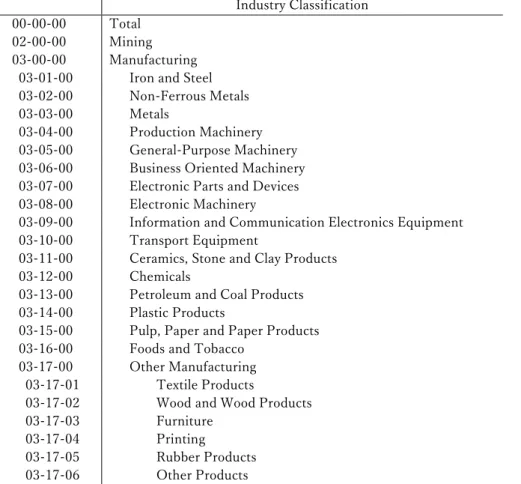
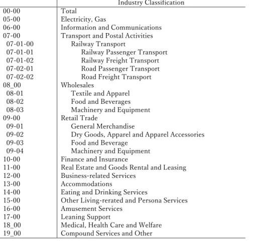
The macroeconomic variables in this study include an index of industrial production, index of tertiary (service) production, private consumption of durable and non-durable goods, private investment of housing and capital, import, and export. Monthly indices of industry and tertiary (service) production are published from the Ministry of Economy, Trade and Industry in Japan.
They are the 2015-based year and seasonally adjusted. The industry classification used in our model is shown in Table 1.
=== Table 1 ===
=== Table 2 ===
As for the private consumption of durable, we substitute the number of new passenger cars registered in Japan, which is published by the Japan Automobile Dealers Association. The data of non-durable private consumption is the number of monthly sales published by the Japan Department Stores Association and by the National Supermarket Association of Japan.
Next, we suppose that the number of housing starts could reflect the current condition of private residential investment. Hence, we utilize historical new construction starts of housing
data which comes from the Ministry of Land, Infrastructure, Transport, and Tourism. The capital investment is substituted for the number of machinery orders from the private sector published by the Economic and Social Research Institute Cabinet Office, Japanese Government.
Price in our model are data of producer price indices and services producer price indices which come from Bank of Japan, consumer price index published in Statics Bureau of Ministry of Internal Affairs and Communications in Japan. The industry classification of producer price indices and services producer price indices corresponds to the classification of the indexes of industrial production, the index of tertiary (service) production.
The data by the industry of wage, employment, and working time come from Monthly Labour Survey published in Ministry of Health, Labour and Welfare in Japan. Our model uses their data about establishments with 30 or more regular employees.The industry classification of these data corresponds to classification of the indexes of industrial production, the index of tertiary (service) production. Then, the data of the long-term interest rate (10 Year’s government bonds yields) of the US is gathered from the Federal Reserve Bank of St. Louis database.
Our model uses the Tokyo Stock Price Index (TOPIX) as the benchmark of the stock price in Japan. We download it from Yahoo Finance. As for data of trade (export/import), the import and export index (quantum) published by Trade Statistics of Japan is utilized in our model.
The COVID-19 Data
We use all data about SIR from the Ministry of Health, Labour and Welfare in Japan: the number of new positive PCR test cases, the number of recoveries from COVID-19, and the number of deaths due to COVID-19. We also utilize COVID-19 Community Mobility Reports by Google to grasp people’s activity in response to before and after COVID-19. In particular, we use data “Residential” in the Google mobility reports. “Residential" shows category shows a change in the duration of time spent at home.
4 Empirical Results
4.1 Estimation Results
As for our economic model, the sample period is from the period January 2016 to October 2020, including 58 observations. Also, the extended SIR model is for January 1, 2020-December 31, 2020. In the framework, most equations are estimated by applying ordinary least squares.
The others are estimated by assuming the Auto-regressive model AR(1), which depends linearly on its previous values and stochastic term. In this section, the results of the estimation and final test are shown. We show several estimation results about crucial variables below.
The Extended SIR Model
Tables 3 and 4 represent the estimated results of the SIR model. We run ordinal least squares to estimate them. In Table 3, the estimated result of equation (5) is shown. We can see the valid relation between (𝐼𝐼𝑡𝑡+1− 𝐼𝐼𝑡𝑡) and 𝑆𝑆𝑡𝑡*𝐼𝐼𝑡𝑡. Although a change in the duration of time spent at home (the Google mobility reports) might be less statistically significant, the result is well estimated.
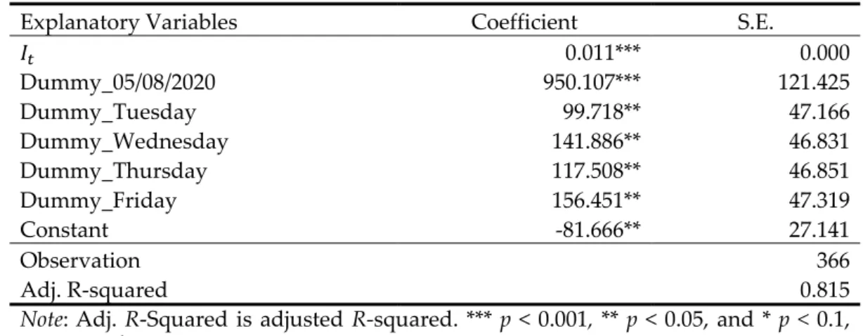
We conclude that it is acceptable. Table 4 displays the result of equation (7). We can see the correlation between the number of recovered/removed persons and infectious persons. This is well estimated.
=== Table 3 ===
=== Table 4 ===
Transmission Rate 𝜷𝜷𝒕𝒕 and Recovery/Remove Rate 𝜸𝜸𝒕𝒕
We can calculate the time-variant parameters of the effective transmission rate 𝛽𝛽𝑡𝑡 and the recovery/remove rate 𝛾𝛾𝑡𝑡 by using estimated parameters, following equations (6) and (8) respectively. Figures 1 and 2 display estimated parameters 𝛽𝛽𝑡𝑡 and 𝛾𝛾𝑡𝑡.
=== Figure 1 ===
Here, considering the relation of 𝐼𝐼𝑡𝑡−1− 𝐼𝐼𝑡𝑡 =𝛽𝛽𝑆𝑆𝑡𝑡𝐼𝐼𝑡𝑡− 𝛾𝛾𝑡𝑡𝐼𝐼𝑡𝑡 in equation (3), 𝛽𝛽𝑆𝑆𝑡𝑡− 𝛾𝛾>0 implies that the epidemic transmission spreads. In the contrast, 𝛽𝛽𝑆𝑆𝑡𝑡− 𝛾𝛾<0 means that infection tends to calm down. Hence, we can see 𝛽𝛽𝑆𝑆𝑡𝑡− 𝛾𝛾𝑡𝑡 as an increasing or decreasing index of the infection.
Figure 2 represents 𝛽𝛽𝑆𝑆𝑡𝑡− 𝛾𝛾. During the first state of emergency, the line is the downward-slope.
It implies that the infection is decreasing. However, the positive values mean that the epidemic doesn’t tend to settle down enough yet.
=== Figure 2 ===
Economic Model
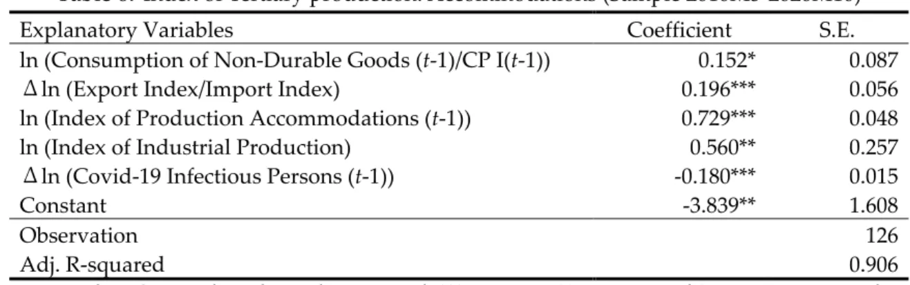
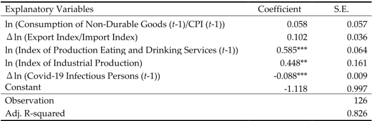
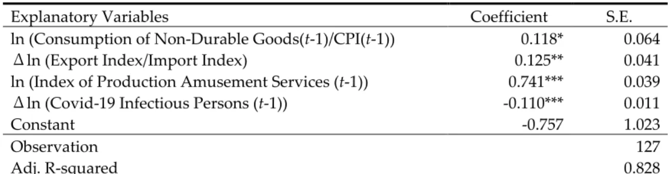
Several estimation results about crucial variables are shown. Tables 5 displays the estimation results of the producer price index of the transport equipment industry. Tables 5, 6, and 7 display the estimation results of the index of tertiary production: accommodations, eating and drinking Services, and amusement services respectively. The results suggest that there is a valid relationship between the number of infectious persons and production. In particular, comparing with coefficients about the number of infectious persons among these industries, we can see that the spread of COVID-19 affects accommodation and amusement service much more negatively.
We estimated all equations, following the framework in the previous section. Some results for stochastic equations, which are not sufficiently satisfactory or show a wrong sign, are
modified or excluded from our system.
=== Table 5 ===
=== Table 6 ===
=== Table 7 ===
=== Table 8 ===
4.2 Final Test
We conducted the final test in order to evaluate the accuracy of our whole system. Some stochastic equations, which worse the performance of the overall system, are excluded from our system, leading to being treated as exogenous variables4. As a result, our simultaneous economic system liked with the extended SIR model consists of 380 simultaneous equations. The modified SIR model includes 7 endogenous equations, where three equations are 𝑆𝑆𝑡𝑡 , 𝐼𝐼𝑡𝑡 , and 𝑅𝑅𝑡𝑡 , two equations are 𝛽𝛽𝑡𝑡 and 𝛾𝛾𝑡𝑡, and the other two are equations bridging two models.
The overall performance of these variables is acceptable. Thus, the estimated results suggest that our theoretical approach has grasped.
It is a challenge to capture the high-frequency fluctuations and to link with two models with different time-periods (monthly-daily). Thus, we conclude that this whole system is acceptable as the first step of our research.
4.3 Scenario Analysis
Now, Japan is under the second state of emergency. Japanese are urged to refrain from going outside unnecessarily and restaurants and shops are asked to shorten their opening hours. This has enabled us to avoid an explosive rise in the number of infections and to suppress surging coronavirus cases. However, the pace of decline has been slowing down. Some ask if self- restraint has worked to prevent the further spread of infections.
In order to reassess the impact of the state of emergency on the Japanese economy as well as the infection, we focus on the first state of emergency. We prepared three scenarios.
Scenario 1:It is assumed that the first state of emergency was implemented until 31 July, on the condition that more strictly self-restraint is imposed until 30 June, and then self-restraint at the level as it was (the first state of emergency that we experienced)
is implemented until 31 July 2020.
Scenario 2:It is assumed that the first state of emergency imposed more strictly self-restraint is implemented until 30 June 2020.
Scenario 3:It is assumed that the state of emergency (self-restraint) at the level as it was (the first state of emergency that we experienced) was extended until 31 July 2020.
Scenario 1 is the most severe self-restraint measures among the three scenarios. All three scenarios are simulated from May 2020 to October 20205. Several crucial results about the three scenarios simulation are shown below.
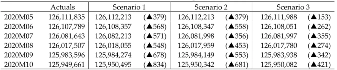
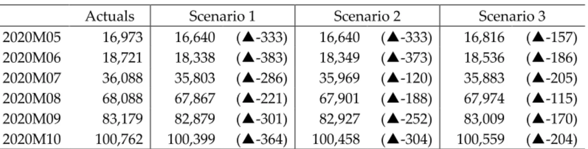
COVID-19 Infection
Figure 3 shows that each scenario simulation leads to changes in the duration of time staying at home. Under these different conditions by scenario, Tables 4, 5, and 6 illustrate changes in the number of susceptible persons, infectious persons, and recovered persons, respectively.
=== Figure 3 ===
We can see that scenario 1 among scenarios can prevent the spread of infection effectively.
Table 9 represents that strict self-restraint like scenarios 1 and 2 may enable to decrease around three hundred infectious persons more than actual values. On the contrary, the results of scenario 3 in Table 9 suggest that even if the state of emergency was extended to July, the monthly reduction of infectious persons is at most less than two hundred.
=== Table 9 ===
=== Table 10 ===
=== Table 11 ===
The Economy
Next, we look at an impact on the economy. Table 12 reports the impacts of the reduction of infections by the enhanced state of emergency on the production of manufacturing and service industries. Manufacturing industries recover after July whereas production of service industries falls in all time periods. One reason for the earlier recovery of manufacturing industries is that the reduction of infectious people has a positive impact on economic activity. However, service industries that rely heavily on in-person interaction tend to continue suffering from the negative economic impact of the COVID-19.
5 Due to data unavailability, we could not simulate analysis after October 2020.
=== Table 12 ===
Furthermore, seeing results by sector, the situation varies. Production of iron and steel industry, one of the key industries in Japan, falls from 2 percent to more than 3 percent at worst under all three scenarios. Production of transport equipment also falls because the demand for mobility is decreasing by public transportations. In contrast, the production of Information and Communication Electronics Equipment increase the production. This is because remote-working and remote-learning increase demand for utilization of electronic communication, leading to increasing the production of information and communication electronics equipment.
=== Table 13 ===
Next, Table 14 shows economic impact of the state of emergency by scenario on production of service industries. It is obvious that accommodation, eating and drinking service, and amusement services, which rely heavily on face-to-face communication or physically close- contact, suffer from significant negative impacts.
=== Table 14 ===
In Table 15, we can see how great the level of the state of emergency give an economic impact on private consumption. Consumption of non-durable goods of supermarket shows positive values. There are two reasons. One is that the supermarkets are classified as an “essential service”
for our daily life. The other is that they have introduced and expanded their online delivery service which allows shopping at home.
=== Table 15 ===
Table 16 shows that the working time of information and communication service increases whereas accommodation and eating and drinking service decline. These results suggest that introducing remote-work and remote-learning stimulate demand for information and communication service. Besides, Table 17 reports the impacts of state of emergency measures on wage rate by sector. Although manufacturing and service industries have negative impacts on their wages, the wage rate of retail trades rises.
=== Table 16 ===
=== Table 17 ===
Considering simulation results, it is found that strengthening or prolonging the state emergency that requests “self-restraint” is effective to some extent to prevent the spread of the infection.
On the other hand, the economic impacts of the implementation of emergency measures consistent a decline in production growth and consumption. However, its economic impacts vary across industries and firms. As for production, service industries are directly affected by containment measures. In particular, the accommodation, food service, and amusement services sectors, which rely heavily on physically close contact, undergo a significant negative impact.
The related industries to service sectors like transport equipment manufacturing, also affect production negatively. In contrast, remote-working and remote learning stimulate the demand for communication equipment, resulting in a great increase in the production of related manufacturing industries. Thus, as negative impacts are offset by positive ones each other, the severe economic slowdown hardly appears in the macroeconomic data explicitly.
However, considering not much difference among scenarios, our simulation results suggest that the measure relying only on “self-restraint” has limited effects. It would be difficult to reduce the infection rate anymore as long as we haven’t had any ways to dies out the infection completely yet. Thus, we think that we are required to promoting more effective measures with various aspects: increasing supplies of vaccines promptly, enhancing active epidemiological surveys, strengthening PCR tests, and increasing bed capacity.
5 Conclusion
This study constructed Japan’s econometric model linked to the extended epidemic SIR model. By implementing scenario simulation analysis, we investigated the effect of the state of emergency that relies on “self-restraint”. The findings are summarized as follows:
1. As for production, service industries are directly affected by containment measures. In particular, the accommodation, food service, and amusement services sectors, which rely heavily on physically close contact, undergo significant negative impacts. The related industries to service sectors like transport equipment manufacturing, also affect production negatively.
2. In contrast, remote-working and remote learning stimulate the demand for communication equipment and its service, resulting in a great increase in the production of related manufacturing industries and service industries.
3. The state of emergency measures has a certain effect on suppressing the increase in the number of infected people. However, considering not much difference among scenarios, our simulation results suggest that the measure relying only on “self-restraint” has limited effects.
Thus, our system constructed the monthly multi-sectoral econometric model linked to the extended epidemic SIR. We also examined the effect of the first state of emergency implemented in April 2020. However, our model requires some improvements. First, infection and recovery rates should be modified to be more structural to explain the effect of other policy measures like increasing supplies of vaccines, enhancing active epidemiological surveys, strengthening PCR tests, and increasing bed capacity. Second, we should extend this model to improve its applicability to policy analysis theoretically and empirically. Our approach is just getting started.
In the future, improving this model would become a more powerful tool and give us better guidance to understand the interaction between epidemic behavior and economic decisions.
References
Alvarez, F., D. Argente, and F. Lippi. (2020), “A Simple Planning Problem for COVID-19 Lockdown,” University of Chicago Becker Friedman Institute for Economics Working Paper, No.
2020-34, 6 April.
Atkeson, A. (2020), “What Will Be The Economic Impact of COVID-19 in the US? Rough Estimates of Disease Scenarios,” EBER Working Paper, No. 26867, March 2020.
Bognanni, M., Hanley, D., Kolliner, D., Mitman, K. (2020), “Economic activity and covid-19 transmission: Evidence from an estimated economic-epidemiological model.”
Eichenbaum, M. S., S. Rebelo, and M. Trabandt. (2020a), “The Macroeconomics of Epidemics,”
NBER Working Paper, No. 26882.
Eichenbaum, M. S., S. Rebelo, and M. Trabandt. (2020b), “The Macroeconomics of Testing and Quarantining,” NBER Working Paper, No. 27104.
Farboodi, M., G. Jarosch, and R. Shimer. (2020), “Internal and External Effects of Social Distancing in a Pandemic,” Covid Economics, Vetted and Real-Time Papers, No. 9, 25–61.
Fujii, F., and T. Nakata. (2020), “Covid-19 and Output in Japan,” RIETI Discussion Paper, Series 21-E-004, January 2021.
Fuss, M. (1977), “The Structure of Technology over Time," Econometrica, Vol. 45(8), 1797-1821 Glover, A., J. Heathcote, D. Krueger, and J-V Rios-Rull. (2020), “Health versus Wealth: On the
Distribution Effects of Controlling a Pandemic,” CERP Discussion Paper, No. 14606, University of Pennsylvania, 2020.
Holtemoller, O. (2020), “Integrated assessment of epidemic and economic dynamics,” IWH Discussion Papers, 4/2020, Halle Institute for Economic Research (IWH).
Kermack, W.O. and McKendrick. A. G. (1927), “Contributions to the mathematical theory of epidemics,” Proceeding of the Royal Society of London, Series A 115, No.772, 7000-721.
Kosaka, H. (2017), “Monthly Econometric Skelton Model,”SFC Discussion Papers, SFC-RM 2017- 001.
Nakamura, S. (1990), “A Nonhomothetic Generalized Leontief Cost Function based on Pooled
Data”, Review of Economics and Statistics, Vol. 72, 649–656.
Negishi, T. (1961), "Monopolistic Competition and General Equilibrium," Review of Economic Studies, Oxford University Press, Vol. 28(3), 196-201.
Table 1. Industry Classification of Index of Industry Production
Industry Classification 00-00-00 Total
02-00-00 Mining 03-00-00 Manufacturing
03-01-00 Iron and Steel 03-02-00 Non-Ferrous Metals 03-03-00 Metals
03-04-00 Production Machinery 03-05-00 General-Purpose Machinery 03-06-00 Business Oriented Machinery 03-07-00 Electronic Parts and Devices 03-08-00 Electronic Machinery
03-09-00 Information and Communication Electronics Equipment 03-10-00 Transport Equipment
03-11-00 Ceramics, Stone and Clay Products 03-12-00 Chemicals
03-13-00 Petroleum and Coal Products 03-14-00 Plastic Products
03-15-00 Pulp, Paper and Paper Products 03-16-00 Foods and Tobacco
03-17-00 Other Manufacturing 03-17-01 Textile Products
03-17-02 Wood and Wood Products 03-17-03 Furniture
03-17-04 Printing
03-17-05 Rubber Products 03-17-06 Other Products
Table 2. Industry Classification of index of Tertiary Industry
Industry Classification
00-00 Total
05-00 Electricity, Gas
06-00 Information and Communications 07-00 Transport and Postal Activities
07-01-00 Railway Transport
07-01-01 Railway Passenger Transport 07-01-02 Railway Freight Transport 07-02-01 Road Passenger Transport 07-02-02 Road Freight Transport
08_00 Wholesales
08-01 Textile and Apparel 08-02 Food and Beverages 08-03 Machinery and Equipment
09-00 Retail Trade
09-01 General Merchandise
09-02 Dry Goods, Apparel and Apparel Accessories 09-03 Food and Beverage
09-04 Machinery and Equipment 10-00 Finance and Insurance
11-00 Real Estate and Goods Rental and Leasing 12-00 Business-related Services
13-00 Accommodations
14-00 Eating and Drinking Services
15-00 Other Living-rerated and Persona Services 16-00 Amusement Services
17-00 Leaning Support
18_00 Medical, Health Care and Welfare 19_00 Compound Services and Other
Table 3. Estimation Result of Susceptible Equation: Sample 01/01/2020-12/31/2020
Explanatory Variables Coefficient S.E.
𝑆𝑆𝑡𝑡*𝐼𝐼𝑡𝑡 -1.37E-10*** 7.46E-12
The number of PCR tests (t-2) -0.032*** 0.004
D(Google_ Residential) 15.297 9.275
Dummy_05082020 -804.758*** 231.892
Dummy_Monday 222.182* 82.182
Dummy_Sunday 376.594*** 83.073
Dummy_PCR 3486.406*** 647.876
Observation 366
Adj. R-squared 0.861
Note: Adj. R-Squared is adjusted R-squared. *** p < 0.001, ** p < 0.05, and * p < 0.1, respectively.
Table 4. Estimation Result of Recovered Equation: Sample 01/01/2020-12/31/2020
Explanatory Variables Coefficient S.E.
𝐼𝐼𝑡𝑡 0.011*** 0.000
Dummy_05/08/2020 950.107*** 121.425
Dummy_Tuesday 99.718** 47.166
Dummy_Wednesday 141.886** 46.831
Dummy_Thursday 117.508** 46.851
Dummy_Friday 156.451** 47.319
Constant -81.666** 27.141
Observation 366
Adj. R-squared 0.815
Note: Adj. R-Squared is adjusted R-squared. *** p < 0.001, ** p < 0.05, and * p < 0.1, respectively.
Table 5. Index of Industrial Production: Transport Equipment Industry (Sample 2016M1-2020M10)
Explanatory Variables Coefficient S.E.
ln (Consumption of Durable Goods-Cars) 0.062 0.036
Δln (Private Housing Investment (t-1)) 0.320* 0.166 Δln (Export Index (t-1)/Import Index (t-1)) 0.052* 0.046 ln(Index of Production Transport Equipment (t--1)) 0.766 0.055 Δln (Index of Tertiary production) 2.067*** 0.349 Δln (Covid-19 Infectious Persons (-2)) -0.054*** 0.010
Constant 0.313 0.416
Observation 58
Adj. R-squared 0.894
Note: Adj. R-Squared is adjusted R-squared. *** p < 0.001, ** p < 0.05, and * p < 0.1, respectively.
Table 6. Index of Tertiary production: Accommodations (Sample 2010M5-2020M10)
Explanatory Variables Coefficient S.E.
ln (Consumption of Non-Durable Goods (t-1)/CP I(t-1)) 0.152* 0.087 Δln (Export Index/Import Index) 0.196*** 0.056 ln (Index of Production Accommodations (t-1)) 0.729*** 0.048
ln (Index of Industrial Production) 0.560** 0.257
Δln (Covid-19 Infectious Persons (t-1)) -0.180*** 0.015
Constant -3.839** 1.608
Observation 126
Adj. R-squared 0.906
Note: Adj. R-Squared is adjusted R-squared. *** p < 0.001, ** p < 0.05, and * p < 0.1, respectively.
Table 7. Index of Tertiary production: Eating and Drinking Services (Sample 2010M5-2020M10)
Explanatory Variables Coefficient S.E.
ln (Consumption of Non-Durable Goods (t-1)/CPI (t-1)) 0.058 0.057 Δln (Export Index/Import Index) 0.102 0.036 ln (Index of Production Eating and Drinking Services (t-1)) 0.585*** 0.064
ln (Index of Industrial Production) 0.448** 0.161
Δln (Covid-19 Infectious Persons (t-1)) -0.088*** 0.009
Constant -1.118 0.997
Observation 126
Adj. R-squared 0.826
Note: Adj. R-Squared is adjusted R-squared. *** p < 0.001, ** p < 0.05, and * p < 0.1, respectively.