An empirical analysis of the money demand function in India

(1)

An empirical analysis of the money demand function in India

著者 Inoue Takeshi, Hamori Shigeyuki

権利 Copyrights 日本貿易振興機構（ジェトロ）アジア

経済研究所 / Institute of Developing

Economies, Japan External Trade Organization (IDE‑JETRO) http://www.ide.go.jp

journal or

publication title

IDE Discussion Paper

volume 166

year 2008‑09‑01

URL http://hdl.handle.net/2344/783

(2)

INSTITUTE OF DEVELOPING ECONOMIES

IDE Discussion Papers are preliminary materials circulated to stimulate discussions and critical comments

Keywords: cointegration, DOLS, India, money demand JEL classification: E41, E52

* Institute of Developing Economies (takeshi_inoue@ide.go.jp).

** Faculty of Economics, Kobe University (hamori@econ.kobe-u.ac.jp).

IDE DISCUSSION PAPER No. 166

An Empirical Analysis of the Money Demand Function in India

Takeshi INOUE * and Shigeyuki HAMORI **

September 2008

Abstract

This paper empirically analyzes India’s money demand function during the period of 1980 to 2007 using monthly data and the period of 1976 to 2007 using annual data. Cointegration test results indicated that when money supply is represented by M1 and M2, a cointegrating vector is detected among real money balances, interest rates, and output. In contrast, it was found that when money supply is represented by M3, there is no long-run equilibrium relationship in the money demand function. Moreover, when the money demand function was estimated using dynamic OLS, the sign conditions of the coefficients of output and interest rates were found to be consistent with theoretical rationale, and statistical significance was confirmed when money supply was represented by either M1 or M2. Consequently, though India’s central bank presently uses M3 as an indicator of future price movements, it is thought appropriate to focus on M1 or M2, rather than M3, in managing monetary policy.

(3)

The Institute of Developing Economies (IDE) is a semigovernmental, nonpartisan, nonprofit research institute, founded in 1958. The Institute merged with the Japan External Trade Organization (JETRO) on July 1, 1998.

The Institute conducts basic and comprehensive studies on economic and related affairs in all developing countries and regions, including Asia, the Middle East, Africa, Latin America, Oceania, and Eastern Europe.

The views expressed in this publication are those of the author(s). Publication does not imply endorsement by the Institute of Developing Economies of any of the views expressed within.

INSTITUTE OF DEVELOPING ECONOMIES (IDE), JETRO 3-2-2, WAKABA,MIHAMA-KU,CHIBA-SHI

CHIBA 261-8545, JAPAN

No part of this publication may be reproduced without the prior permission of the IDE-JETRO.

(4)

An Empirical Analysis of the Money Demand Function in India

Inoue Takeshi

(Institute of Developing Economies) and

Shigeyuki Hamori

(Faculty of Economics, Kobe University)

Abstract

This paper empirically analyzes India’s money demand function during the period of 1980 to 2007 using monthly data and the period of 1976 to 2007 using annual data. Cointegration test results indicated that when money supply is represented by M1 and M2, a cointegrating vector is detected among real money balances, interest rates, and output. In contrast, it was found that when money supply is represented by M3, there is no long-run equilibrium relationship in the money demand function. Moreover, when the money demand function was estimated using dynamic OLS, the sign conditions of the coefficients of output and interest rates were found to be consistent with theoretical rationale, and statistical significance was confirmed when money supply was represented by either M1 or M2. Consequently, though India’s central bank presently uses M3 as an indicator of future price movements, it is thought appropriate to focus on M1 or M2, rather than M3, in managing monetary policy.

JEL classification : E41; E52

Keywords : Cointegration; DOLS; India; Money Demand

(5)

1. Introduction

In India, financial sector deregulation was undertaken beginning in the mid-1980s, when steps like the introduction of 182-day Treasury bills, lifting of the call money interest-rate ceiling, and the introduction of certificates of deposit and commercial paper were taken in a bid to make the government securities market and the money market more efficient (Sen and Vaidya 1997 [18]). Furthermore, with the balance of payments crisis in 1991, there began an intermittent series of more systematic financial sector reforms that continues even today. For example, the reform of the Indian interest-rate structure, which had been strictly managed by the Reserve Bank of India (RBI), began with the April 1992 deregulation of deposit rates and has progressed to the point where commercial banks are now permitted to freely set term deposit rates and lending rates for loans above Rs.2 lakh.¹ Moreover, the RBI, which had long been constrained by the Indian government's fiscal management, entered into an agreement with the government in September 1994 to limit the issuance of 91-day ad hoc Treasury bills, which were used to finance fiscal deficits, and eventually eliminated these securities altogether in April 1997, greatly reining in the central bank's automatic monetization of fiscal deficits.²

The above are just a few examples of how interest-rate structure deregulation and the introduction of new financial products have progressed in India over the past 20 years.

Theoretical research and empirical analyses, using primarily data on developed countries, have shown that the money demand function can become unstable as a result of such financial innovations and financial sector reforms. Partly because of instability in the money demand function, many central banks have in recent years switched from money supply targeting focused on monetary aggregates as the intermediate target, to inflation targeting, which seeks to stabilize prices by adjusting interest rates based on inflation forecasts. The RBI abandoned the flexible monetary targeting approach in favor of the multiple indicator approach in April 1998, putting an end to the use of money supply as the intermediate target, but retaining it as an important indicator of future prices. Consequently, examining the characteristics of the money demand function of India's financial sector, which has undergone significant change since the 1980s, should bear significant meaning for present and future considerations of the RBI’s monetary policy. This paper, therefore, uses annual data for the period of 1976 to 2007 and monthly data for the period of January 1980 to December 2007 to estimate India's money

1 Except for bank savings deposits, non-resident deposits, loans for less than 200,000 rupees, and export credit, interest rates have been greatly deregulated.

2 Financial deregulation beginning in the 1990s also loosened requirements, like those requiring commercial banks to keep central bank balances equal to a certain percentage of their own deposits and purchase government bonds and government-specified bonds, and the deregulation relaxed barriers to entering the banking sector and opened stock markets to foreign participants.

(6)

demand function, which is derived from real money balances, interest rates, and output, and shed light on its characteristics.

The next section of this paper consists of a review of relevant prior research and a discussion of the unique contributions of this paper. In the third section, the models are presented and in the fourth section, variables are defined, sources are provided, and data characteristics are explained.

Moving into the fifth section, cointegration tests are performed using both monthly and annual data, the long-term stability of the money demand function is examined, and dynamic OLS (DOLS) is used to examine the sign conditions and significance of output and interest-rate coefficients. Lastly, analysis results are used to discuss the characteristics of India's money demand function and the implications for India's monetary policy.

2. Literature Review

India's money demand function has been the subject of numerous quantitative research efforts.

Among these was the first study to explicitly consider the stationarity of, and cointegration relationships among, the variables of the money demand function. Moosa (1992) used three types of money supply – cash, M1, and M2 – to perform cointegration tests on real money balances, short-term interest rates, and industrial production over the period beginning with the first quarter of 1972 and extending through the fourth quarter of 1990. Results indicated that for all three types of money supply, the money balance had a cointegrating relationship with output and interest rates. However, greater numbers of cointegrating vectors were detected for cash and M1 than for M2, so Moosa (1992) states that narrower definitions of money supply are better for pursuing monetary policy.

Bhattacharya (1995), like Moosa (1992), considered three types of money supply – M1, M2, and M3 – and used annual data for the period of 1950 to 1980 to analyze India's money demand function. Bhattacharya (1995) performed cointegration tests for real money balances, real GNP, and long-term and short-term interest rates, detected a cointegrating relationship among variables only when money supply was defined as M1, and clearly showed that long-term interest rates are more sensitive to money demand than are short-term interest rates. In addition, Bhattacharya (1995), after estimating an error correction model based on cointegration test results, found that, in the case of M1, the error correction term is significant and negative, and held that monetary policy is stable over the long term when money supply is narrowly defined.

Bahmani-Oskooee and Rehman (2005) analyzed the money demand functions for India and six other Asian countries during the period beginning with the first quarter of 1972 and ending with the fourth quarter of 2000. Using the ARDL approach described in Pesaran et al. (2001),

(7)

they performed cointegration tests on real money supplies, industrial production, inflation rates, and exchange rates (in terms of US dollar). For India, cointegrating relationships were detected when money supply was defined as M1, but not M2, so they concluded that M1 is the appropriate money supply definition to use in setting monetary policy.

Contrasting with the above, there is also prior research that uses money supply defined broadly in holding that India's money demand function is stable. In one example, Pradhan and Subramanian (1997) employed cointegration tests, an error correction model, and annual data for the period of 1960 to 1994 to detect relationships among real money balances, real GDP, and nominal interest rates. They estimated an error correction model using M1 and M3 as money supply definitions and found the error correction term to be significant and negative. Their position, therefore, was that the money demand function is stable not only with M1 but also with M3.

Das and Mandal (2000) considered only the M3 money supply in stating that India's money demand function is stable. They used monthly data for the period of April 1981 to March 1998 to perform cointegration tests and detected cointegrating vectors among money balance, industrial production, short-term interest rates, wholesale prices, share prices, and real effective exchange rates. Their position, therefore, was that long-term money demand relevant to M3 is stable. Similarly, Ramachandran (2004), too, considered only the M3 money supply in using annual data for the period of 1951/52 to 2000/01 to perform cointegration tests on nominal money supply, output, and price levels. Because stable relationships were discovered among these three variables, Ramachandran (2004) states that, over the long term, it is possible to use an increase in M3 as a latent indicator of future price movements.

As is the case with the studies referred to above, prior research in general states that India's money demand function is stable.³ Furthermore, studies performed using multiple money supply definitions have tended to draw the conclusion that because India's money demand function is more stable when money supply is defined narrowly, the central bank should adopt cash or M1 as the narrow definition of money supply when determining monetary policy.

Contrasting with that position, however, other studies have concluded that the money demand function is stable when money supply is broadly defined. Views on what definition of money supply to use for monetary policy, therefore, differ.

This paper uses both monthly and annual data, considers three types of money supply – M1, M2, and M3, and comprehensively estimates India's money demand functions for each case. It

3 Nag and Upadhyay (1993), Parikh (1994), Rao and Shalabh (1995), Rao and Singh (2006), and others as well have also performed quantitative analyses of India’s money demand function.

(8)

also discusses the implications of empirical results for the RBI’s monetary policy formation. In contrast with prior studies, this paper, after performing cointegration tests on money supply, output, and interest rates as money demand function variables, applies DOLS and sheds light on the characteristics of India's money demand function through examinations of the sign conditions and statistical significance of variable coefficients.

3. Models

There are various theories concerning the money demand function. For example, Kimbrough (1986a, 1986b) and Faig (1988) came up with the following money demand function as a result of explicitly considering transaction costs.

( , )

t

t t

t

M L Y R

P ⁼ L^Y >⁰, L_R <0 (1)

In this formula, Mt represents nominal money supply for period t_; P_t represents the price index for period t _;Y_t represents output for period t_{; and}R_t represents the nominal interest rate for period t. Increases in output bring increases in money demand, and increases in interest rates bring decreases in money demand.

We use two models corresponding to equation (1) in order to conduct an empirical analysis.

Model 1: ln(M_t)−ln( )P_t = β₀ +β₁ln( )Y_t +β₂R_t +u_t, β₁ >0,β₂ <0 (2)

Model 2: ln(M_t)−ln( )P_t = β₀ +β₁ln( )Y_t +β₂ln(R_t)+u_t, β₁ >0,β₂ <0 (3)

Both Models (2) and (3) are log linear models, but Model (2) uses the level of interest rates and Model (3) uses the logarithm value of interest rates.

4. Data

This paper uses both monthly data and annual data for empirical analysis. For monthly data, we use data over the period of January 1980 to December 2007. The data source for the industrial production index (seasonally adjusted by X12) and the wholesale price index is IMF (2008). We obtained M1, M2, and M3 from various issues of the RBI Bulletin. We deflate these monetary aggregates by the wholesale price index, and we use the call rate as the interest rate.

(9)

The call rate was obtained from RBI (2006) over the period of January 1980 to December 2005, RBI (2007a) and RBI (2008) over the period of January 2006 to December 2007.

For annual data, we use data over the period of 1976 to 2007. Real GDP and the GDP deflator were taken from IMF (2008). We obtained M1, M2, and M3 from various issues of the RBI Bulletin. We deflate these monetary aggregates by the GDP deflator, and we use the call rate as the interest rate. The call rate was obtained from RBI (2007b) and RBI (2008). Logarithm values are used for money supply, price levels, and output (industrial production and GDP).

Interest rates are analyzed in two ways, taking a logarithm in one case and not in the other.

As a preliminary analysis, we carried out the augmented Dickey-Fuller tests for the logs of real money balances, output, and interest rates (Dickey and Fuller 1979). As a result, the level of each variable was found to have a unit root, whereas the first difference of each variable was found not to have a unit root. Thus, we can say that each variable is a nonstationary variable with a unit root.

5. Empirical Results 5.1 Monthly Data

First, we analyzed the money demand function in relation to the use of M1 using the monthly data over the period of January 1980 to December 2007. For that analysis, we conducted Johansen cointegration tests for the money demand function (Johansen 1991). There are two kinds of Johansen-type tests: the trace test and the maximum eigen-value test.

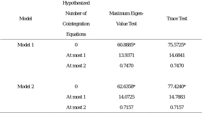
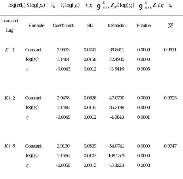
Table 1 shows the results of cointegration tests for Model 1 and Model 2. Model 1 includes the logs of real money balances, the logs of industrial production, and the interest rate; whereas Model 2 includes the logs of real money balances, the logs of industrial production, and the logs of interest rates. As is evident from Table 1, the null hypothesis of no cointegrating relation is rejected at the 5% significance level for both models. As the existence of the cointegrating relation was supported, we estimated the money demand function using dynamic OLS (DOLS).⁴ Table 2 shows the estimation results with respect to Model 1. As is evident from this table, the output coefficient is significantly estimated to be at positive values (1.1484 for K=1, 1.1498 for K=2, and 1.1556 for K=6). The interest rate coefficient is significantly estimated to be at negative values (-0.0043 for K=1, -0.0049 for K=2, and -0.0050 for K=6). Thus, the sign condition of the money demand function holds for all cases. Table 3 shows the estimation results with respect to Model 2. As is evident from this table, the sign condition of the money demand function holds for all cases. The output coefficient was significantly estimated at

4 Standard errors are calculated using the method of Newey and West (1987).

(10)

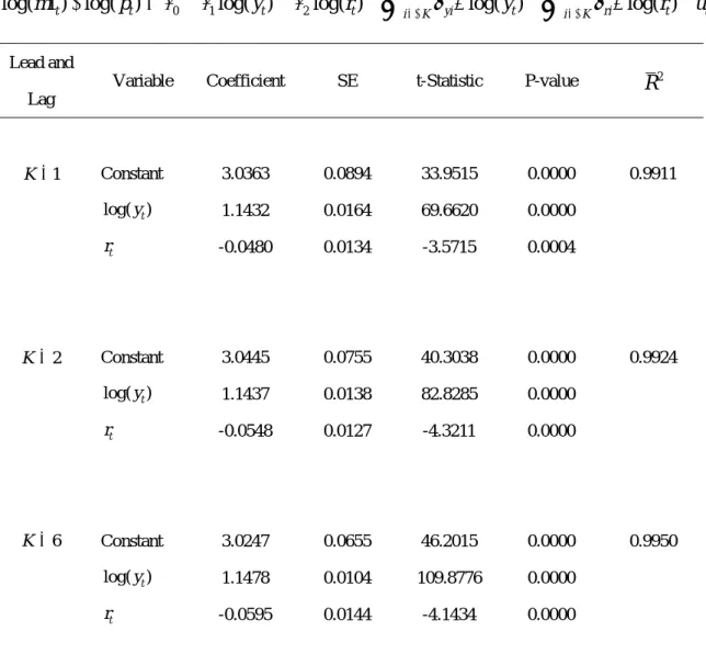
positive values (1.1432 for K=1, 1.1437 for K=2, and 1.1478 for K=6), while the interest rate coefficient was significantly estimated at negative values (-0.0480 for K=1, -0.0548 for K=2, and -0.0595 for K=6). As is evident from the above results, it became clear that a cointegrating relation was supported and that the existence of a money demand function with respect to M1 was statistically supported.

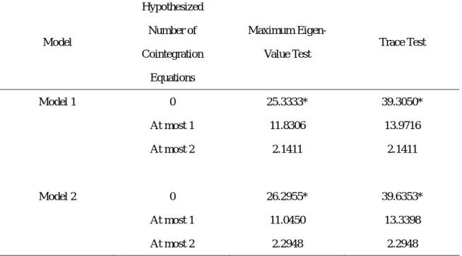
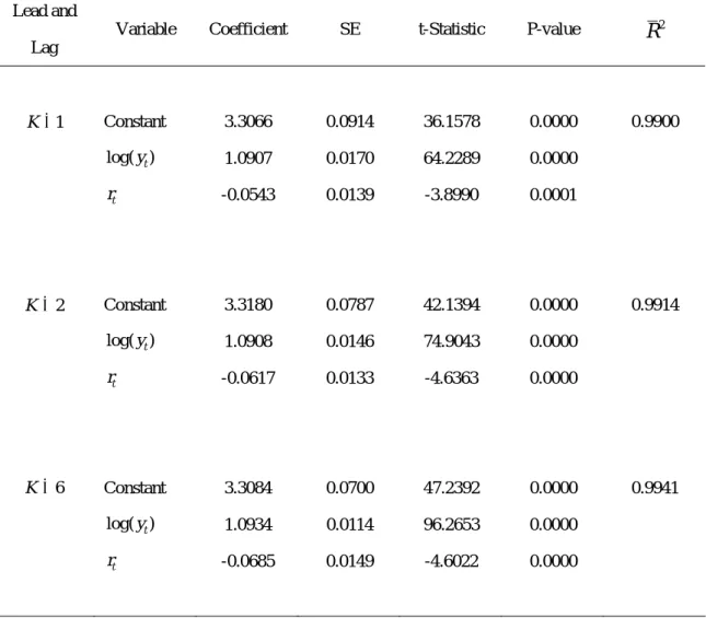
Next, we considered the money demand function when using M2 for the money supply component. Table 4 indicates the results of cointegration tests for Model 1 and Model 2. As is evident from the table, the null hypothesis of no cointegration is rejected at the 5% significance level for both models. As the existence of the cointegrating relation was supported, we estimated the money demand function using DOLS. Table 5 shows the estimation results with respect to Model 1. As is evident from this table, the sign condition of the money demand function holds. The output coefficient was significantly estimated at positive values of 1.0966 for K=1, 1.0977 for K=2, and 1.1023 for K=6, while the interest rate coefficient was significantly estimated at negative values of -0.0049 for K=1, -0.0055 for K=2, and -0.0059 for K=6. Table 6 shows the estimation results with respect to Model 2. As is evident from this table, the sign condition of the money demand function holds. The output coefficient was significantly estimated at positive values of 1.0907 for K=1, 1.0908 for K=2, and 1.0934 for K=6, while the interest rate coefficient was significantly estimated at negative values of -0.0543 for K=1, -0.0617 for K=2, and -0.0685 for K=6. As is evident from the above results, it became clear that a cointegrating relation was supported and that the existence of a money demand function with respect to M2 was statistically supported.

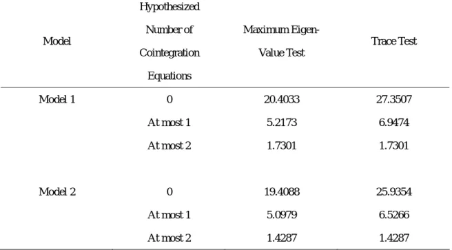
Finally, we considered the money demand function when using M3 for the money supply component. Table 7 indicates the results of cointegration tests for Model 1 and Model 2. As is evident from this table, the null hypothesis (in which there is no cointegrating relation) is not rejected at the 5% significance level for either of the models. It became clear that a cointegrating relation was not supported and thus that the existence of a money demand function with respect to M3 was not statistically supported.

5.2 Annual Data

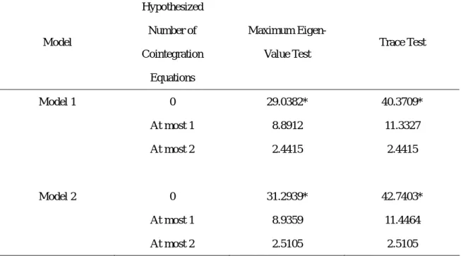
We also analyzed the money demand function in relation to the use of M1 using the annual data over the period from 1976 to 2007. Since industrial production does not necessarily reflect the total level of output in the Indian economy, it is worthwhile to analyze the money demand function using annual data, which enables us to use the GDP data. Table 8 shows the results of cointegration tests for Model 1 and Model 2. As is evident from Table 8, the null hypothesis of

(11)

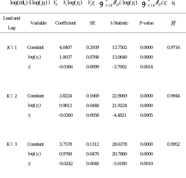
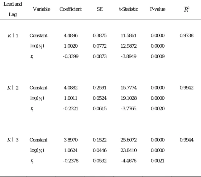
no cointegrating relation is rejected at the 5% significance level for both models. As the existence of the cointegrating relation was supported, we estimated the money demand function using DOLS. Table 9 shows the estimation results with respect to Model 1. As is evident from this table, the output coefficient is significantly estimated to be positive (1.0037 for K=1, 0.9812 for K=2, and 0.9769 for K=3). The interest rate coefficient is significantly estimated to be negative (-0.0366 for K=1, -0.0260 for K=2, and -0.0242 for K=3). Thus, the sign condition of the money demand function holds for all cases. Table 10 shows the estimation results with respect to Model 2. As is evident from this table, the sign condition of the money demand function holds for all cases. The output coefficient was significantly estimated to be positive (1.0020 for K=1, 1.0011 for K=2, and 1.0624 for K=3), while the interest rate coefficient was significantly estimated to be negative (-0.3399 for K=1, -0.2321 for K=2, and -0.2378 for K=3).

As is evident from the above results, it became clear that a cointegrating relation was supported and that the existence of a money demand function with respect to M1 was statistically supported.

Next, we considered the money demand function when using M2 for the money supply component. Table 11 indicates the results of cointegration tests for Model 1 and Model 2. As is evident from the table, the null hypothesis of no cointegration is rejected at the 5% significance level for both models. As the existence of the cointegrating relation was supported, we estimated the money demand function using DOLS. Table 12 shows the estimation results with respect to Model 1. As is evident from this table, the sign condition of the money demand function holds. The output coefficient was significantly estimated at positive values of 0.9402 for K=1, 0.9173 for K=2, and 0.9132 for K=3, while the interest rate coefficient was significantly estimated at negative values of -0.0397 for K=1, -0.0295 for K=2, and -0.0278 for K=3. Table 13 shows the estimation results with respect to Model 2. As is evident from this table, the sign condition of the money demand function holds. The output coefficient was significantly estimated at positive values of 0.9381 for K=1, 0.9374 for K=2, and 0.9988 for K=3, while the interest rate coefficient was significantly estimated at negative values of -0.3669 for K=1, -0.2648 for K=2, and -0.2715 for K=3. As is evident from the above results, it became clear that a cointegrating relation was supported and that the existence of a money demand function with respect to M2 was statistically supported.

Finally, we considered the money demand function when using M3 for the money supply component. Table 14 indicates the results of cointegration tests for Model 1 and Model 2. As is evident from this table, the null hypothesis (in which there is no cointegrating relation) is not rejected at the 5% significance level in three out of four cases. It became clear that a cointegrating relation may not be supported and thus that the existence of a money demand

(12)

function with respect to M3 may not be statistically supported.

Our empirical results using annual data are consistent with those using monthly data. Thus, the cointegrating relation for the money demand function is statistically supported for M1 and M2, but not for M3 for both monthly and annual data.

6. Some Concluding Remarks

If an equilibrium relationship is observed in the money demand function, financial authorities can employ appropriate money supply controls to maintain a reasonable inflation rate. This paper empirically analyzed India's money demand function over the period of 1980 to 2007 using monthly data and the period of 1976 to 2007 using annual data. Results supported the existence of an equilibrium relation in money demand when money supply was defined as M1 or M2, but no such relation was detected when money supply was defined as M3. These results were obtained for both monthly and annual data, so they were not affected by data intervals and were robust in this sense.

What are the implications of these results for India's monetary policy? In the mid-1980s, the RBI adopted monetary targeting focused on the medium-term growth rate of the M3 money supply. Monetary targeting was used as a flexible policy framework to be adjusted in accordance with changes in production and prices, rather than as a strict policy rule. However, amid ongoing financial innovations and financial sector reforms, the RBI announced in April 1998 that it would switch to the multiple indicator approach in order to be able to consider a wider array of factors in setting policy. Under this new policy framework, the M3 growth rate is used as one reference indicator.

In general, a reference indicator, as an indicator of future economic conditions, is used as something between an operating instrument and a final objective, and no target levels are set, as is the case, for example, with intermediate targets. However, in India, where it is used as a reference indicator, the forecast growth rate for the M3 money supply is publicly announced on an annual basis, and it is focused on as a measure of future price movements. Consequently, Indian financial authorities, despite the fact that they have changed their policy framework, continue to pay significant attention to M3 movements. The empirical results of this paper, though, suggest that the RBI would be able to more appropriately control price levels if it would refer to the M1 and M2, rather than the M3, money supplies in managing monetary policy.

(13)

References

Bahmani-Oskooee, Mohsen, and Hafez Rehman. 2005. "Stability of the Money Demand Function in Asian Developing Countries." Applied Economics 37, no. 7: 773-792.

Bhattacharya, Radha. 1995. "Cointegrating Relationships in the Demand for Money in India."

The Indian Economic Journal 43, no. 1: 69-75.

Das, Samarjit, and Kumarjit Mandal. 2000. "Modeling Money Demand in India: Testing Weak, Strong & Super Exogeneity." Indian Economic Review 35, no. 1: 1-19.

Dickey, David A., and Wayne A. Fuller. 1979. "Distribution of the Estimators for Autoregressive Time Series with a Unit Root." Journal of the American Statistical Association 74, no. 366:

427-431.

Faig, Miquel. 1988. "Characterization of the Optimal Tax on Money when it Functions as a Medium of Exchange." Journal of Monetary Economics 22, no. 1: 137-148.

International Monetary Fund. 2008. International Financial Statistics. Washington, D.C.: IMF, April.

Johansen, Søren. 1991. "Estimation and Hypothesis Testing of Cointegration Vectors in Gaussian Vector Autoregressive Models." Econometrica 59, no. 6: 1551-1580.

Kimbrough, Kent P. 1986a. "Inflation, Employment, and Welfare in the Presence of Transactions Costs." Journal of Money, Credit, and Banking 18, no. 2: 127-140.

Kimbrough, Kent P. 1986b. "The Optimum Quantity of Money Rule in the Theory of Public Finance." Journal of Monetary Economics 18, no. 3: 277-284.

Moosa, Imad. 1992. "The Demand for Money in India: A Cointegration Approach." The Indian Economic Journal 40, no. 1: 101-115.

Nag, Ashok K., and Ghanshyam Upadhyay. 1993. "Estimating Money Demand Function: A Cointegration Approach." Reserve Bank of India Occasional Papers 14, no. 1: 47-66.

Newey, Whitney and Kenneth, West. 1987. "A Simple Positive Semi-Definite, Heteroskedasticity and Autocorrelation Consistent Covariance Matrix." Econometrica 55, no.3: 703–708.

Parikh, Ashok. 1994. "An Approach to Monetary Targeting in India." Reserve Bank of India Development Research Group Study, no. 9, October.

Pesaran, M. H., Y. Shin, and R. J. Smith. 2001. "Bounds Testing Approaches to the Analysis of Level Relationships." Journal of Applied Econometrics 16, no. 3: 289-326.

Pradhan, B. K., and A. Subramanian. 1997. "On the Stability of the Demand for Money in India." The Indian Economic Journal 45, no. 1: 106-117.

Ramachandran, M. 2004. "Do Broad Money, Output, and Prices Stand for a Stable Relationship

(14)

in India?" Journal of Policy Modeling 26, nos. 8-9: 983-1001.

Rao, Bhaskara B., and Shalabh. 1995. "Unit Roots Cointegration and the Demand for Money in India." Applied Economics Letters 2, no. 10: 397-399.

Rao, Bhaskara B., and Rup Singh. 2006. "Demand for Money in India: 1953-2003." Applied Economics 38, no. 11: 1319-1326.

Reserve Bank of India. 2006. Handbook of Monetary Statistics of India. Mumbai: RBI, March.

Reserve Bank of India. 2007a. Macroeconomic and Monetary Developments First Quarter Review 2007-08. Mumbai: RBI, July.

Reserve Bank of India. 2007b. Handbook of Statistics on Indian Economy. Mumbai: RBI, October.

Reserve Bank of India. 2008. Macroeconomic and Monetary Developments in 2007-08.

Mumbai: RBI, April.

Reserve Bank of India. various issues. RBI Bulletin. Mumbai: RBI.

Sen, Kunal, and Rajendra R. Vaidya. 1997. The Process of Financial Liberalization. Delhi:

Oxford University Press.

(15)

Table 1 Cointegration Tests (M1, Monthly data)

* indicates that the null hypothesis is rejected at the 5% significance level.

Model

Hypothesized Number of Cointegration

Equations

Maximum Eigen- Value Test

Trace Test

Model 1 0 60.8885* 75.5725*

At most 1 13.9371 14.6841

At most 2 0.7470 0.7470

Model 2 0 62.6358* 77.4240*

At most 1 14.0725 14.7883

At most 2 0.7157 0.7157

(16)

Table 2 Dynamic OLS (M1, Monthly data, Model 1)

0 1 2

log( 1 ) log(

_t _t

) log( )

_t _t ^K _yi

log( )

_t ^K _ri _t _t

i K i K

m − p =

β

+

β

y +

β

r +

∑

₌₋

γ

Δ y +

∑

₌₋

γ

Δ +r u

Lead and Lag

Variable Coefficient SE t-Statistic P-value R²

1

K= Constant 2.9533 0.0741 39.8611 0.0000 0.9911 log( )y_t 1.1484 0.0158 72.4935 0.0000

rt -0.0043 0.0012 -3.5416 0.0005

2

K= Constant 2.9478 0.0626 47.0700 0.0000 0.9923 log( )y_t 1.1498 0.0135 85.2199 0.0000

rt -0.0049 0.0012 -4.0843 0.0001

6

K= Constant 2.9130 0.0539 54.0741 0.0000 0.9947 log( )y_t 1.1556 0.0107 108.2575 0.0000

rt -0.0050 0.0015 -3.3923 0.0008

Note: SE is the Newy-West HAC Standard Error (lag truncation=5).

(17)

0 1 2

log( 1 ) log(

_t _t

) log( )

_t

log( )

_t ^K _yi

log( )

_t ^K _ri

log( )

_t _t

i K i K

m − p =

β

+

β

y +

β

r +

∑

₌₋

γ

Δ y +

∑

₌₋

γ

Δ r +u

Lead and

Lag

1

K= Constant 3.0363 0.0894 33.9515 0.0000 0.9911 log( )y_t 1.1432 0.0164 69.6620 0.0000

rt -0.0480 0.0134 -3.5715 0.0004

2

K= Constant 3.0445 0.0755 40.3038 0.0000 0.9924 log( )y_t 1.1437 0.0138 82.8285 0.0000

rt -0.0548 0.0127 -4.3211 0.0000

6

K= Constant 3.0247 0.0655 46.2015 0.0000 0.9950 log( )y_t 1.1478 0.0104 109.8776 0.0000

rt -0.0595 0.0144 -4.1434 0.0000

(18)

Model

Equations

Trace Test

Model 1 0 25.3333* 39.3050*

At most 1 11.8306 13.9716

At most 2 2.1411 2.1411

Model 2 0 26.2955* 39.6353*

At most 1 11.0450 13.3398

At most 2 2.2948 2.2948

(19)

0 1 2

log( 2 ) log(

_t _t

) log( )

_t _t ^K _yi

log( )

_t ^K _ri _t _t

i K i K

m − p =

β

+

β

y +

β

r +

∑

₌₋

γ

Δ y +

∑

₌₋

γ

Δ +r u

Lead and Lag

1

K= Constant 3.2129 0.0760 42.2970 0.0000 0.9899 log( )y_t 1.0966 0.0165 66.5934 0.0000

rt -0.0049 0.0012 -3.9508 0.0001

2

K= Constant 3.2096 0.0655 49.0098 0.0000 0.9913 log( )y_t 1.0977 0.0143 76.7408 0.0000

rt -0.0055 0.0012 -4.5206 0.0000

6

K= Constant 3.1817 0.0583 54.5536 0.0000 0.9938 log( )y_t 1.1023 0.0117 94.5821 0.0000

rt -0.0059 0.0015 -3.8277 0.0002

(20)

0 1 2

log( 2 ) log(

_t _t

) log( )

_t

log( )

_t ^K _yi

log( )

_t ^K _ri

log( )

_t _t

i K i K

m − p =

β

+

β

y +

β

r +

∑

₌₋

γ

Δ y +

∑

₌₋

γ

Δ r +u

Lead and Lag

1

K= Constant 3.3066 0.0914 36.1578 0.0000 0.9900 log( )y_t 1.0907 0.0170 64.2289 0.0000

rt -0.0543 0.0139 -3.8990 0.0001

2

K= Constant 3.3180 0.0787 42.1394 0.0000 0.9914 log( )y_t 1.0908 0.0146 74.9043 0.0000

rt -0.0617 0.0133 -4.6363 0.0000

6

K= Constant 3.3084 0.0700 47.2392 0.0000 0.9941 log( )y_t 1.0934 0.0114 96.2653 0.0000

rt -0.0685 0.0149 -4.6022 0.0000

(21)

Model

Equations

Trace Test

Model 1 0 20.4033 27.3507

At most 1 5.2173 6.9474

At most 2 1.7301 1.7301

Model 2 0 19.4088 25.9354

At most 1 5.0979 6.5266

At most 2 1.4287 1.4287

(22)

Table 8 Cointegration Tests (M1, Annual data)

Model

Equations

Trace Test

Model 1 0 29.0382* 40.3709*

At most 1 8.8912 11.3327

At most 2 2.4415 2.4415

Model 2 0 31.2939* 42.7403*

At most 1 8.9359 11.4464

At most 2 2.5105 2.5105

(23)

Table 9 Dynamic OLS (M1, Annual data, Model 1)

0 1 2

log( 1 ) log(

_t _t

) log( )

_t _t ^K _yi

log( )

_t ^K _ri _t _t

i K i K

m − p =

β

+

β

y +

β

r +

∑

₌₋

γ

Δ y +

∑

₌₋

γ

Δ +r u

Lead and Lag

1

K= Constant 4.0407 0.2939 13.7502 0.0000 0.9716 log( )y_t 1.0037 0.0768 13.0640 0.0000

rt -0.0366 0.0099 -3.7002 0.0014

2

K= Constant 3.8224 0.1669 22.9069 0.0000 0.9944 log( )y_t 0.9812 0.0448 21.9224 0.0000

rt -0.0260 0.0058 -4.4821 0.0005

3

K= Constant 3.7578 0.1312 28.6378 0.0000 0.9952 log( )y_t 0.9769 0.0470 20.7860 0.0000

rt -0.0242 0.0048 -5.0189 0.0010

(24)

0 1 2

log( 1 ) log(

_t _t

) log( )

_t

log( )

_t ^K _yi

log( )

_t ^K _ri

log( )

_t _t

i K i K

m − p =

β

+

β

y +

β

r +

∑

₌₋

γ

Δ y +

∑

₌₋

γ

Δ r +u

Lead and Lag

1

K= Constant 4.4896 0.3875 11.5861 0.0000 0.9738 log( )y_t 1.0020 0.0772 12.9872 0.0000

rt -0.3399 0.0873 -3.8949 0.0009

2

K= Constant 4.0882 0.2591 15.7774 0.0000 0.9942 log( )y_t 1.0011 0.0524 19.1028 0.0000

rt -0.2321 0.0615 -3.7765 0.0020

3

K= Constant 3.8970 0.1522 25.6072 0.0000 0.9944 log( )y_t 1.0624 0.0446 23.8410 0.0000

rt -0.2378 0.0532 -4.4676 0.0021

(25)

Model

Equations

Trace Test

Model 1 0 29.4465* 40.2924*

At most 1 8.9430 10.8459

At most 2 1.9029 1.9029

Model 2 0 31.8685* 42.6966*

At most 1 8.9294 10.8281

At most 2 1.8988 1.8988

(26)

0 1 2

log( 1 ) log(

_t _t

) log( )

_t _t ^K _yi

log( )

_t ^K _ri _t _t

i K i K

m − p =

β

+

β

y +

β

r +

∑

₌₋

γ

Δ y +

∑

₌₋

γ

Δ +r u

Lead and Lag

1

K= Constant 4.3669 0.2886 15.1317 0.0000 0.9676 log( )y_t 0.9402 0.0760 12.3674 0.0000

rt -0.0397 0.0098 -4.0638 0.0006

2

K= Constant 4.1610 0.1650 25.2232 0.0000 0.9936 log( )y_t 0.9173 0.0443 20.7286 0.0000

rt -0.0295 0.0057 -5.1387 0.0002

3

K= Constant 4.1007 0.1311 31.2843 0.0000 0.9948 log( )y_t 0.9132 0.0478 19.1190 0.0000

rt -0.0278 0.0049 -5.7213 0.0004

(27)

0 1 2

log( 1 ) log(

_t _t

) log( )

_t

log( )

_t ^K _yi

log( )

_t ^K _ri

log( )

_t _t

i K i K

m − p =

β

+

β

y +

β

r +

∑

₌₋

γ

Δ y +

∑

₌₋

γ

Δ r +u

Lead and Lag

1

K= Constant 4.8505 0.3788 12.8058 0.0000 0.9702 log( )y_t 0.9381 0.0757 12.3845 0.0000

log( )r_t -0.3669 0.0857 -4.2806 0.0004

2

K= Constant 4.4693 0.2556 17.4837 0.0000 0.9935 log( )y_t 0.9374 0.0511 18.3566 0.0000

log( )r_t -0.2648 0.0613 -4.31665 0.0007

3

K= Constant 4.2862 0.1556 27.5495 0.0000 0.9938 log( )y_t 0.9988 0.0463 21.5558 0.0000

log( )r_t -0.2715 0.0541 -5.0207 0.0010

(28)

Model

Equations

Trace Test

Model 1 0 20.7221 31.4139*

At most 1 6.7122 10.6918

At most 2 3.9796 3.9796

Model 2 0 18.0444 28.3185

At most 1 6.5157 10.2741

At most 2 3.7584 3.7584