PAPER
An Integrated Method to Remove Color Cast and Contrast Enhancement for Underwater Image
Siaw-Lang WONG†, Raveendran PARAMESRAN†a), Ibuki YOSHIDA††,Nonmembers, andAkira TAGUCHI††b),Fellow
SUMMARY Light scattering and absorption of light in water cause underwater images to be poorly contrasted, haze and dominated by a single color cast. A solution to this is to find methods to improve the quality of the image that eventually leads to better visualization. We propose an integrated approach using Adaptive Gray World (AGW) and Differential Gray-Levels Histogram Equalization for Color Images (DHECI) to remove the color cast as well as improve the contrast and colorfulness of the underwater image.
The AGW is an adaptive version of the GW method where apart from computing the global mean, the local mean of each channel of an image is taken into consideration and both are weighted before combining them. It is applied to remove the color cast, thereafter the DHECI is used to improve the contrast and colorfulness of the underwater image. The results of the proposed method are compared with seven state-of-the-art methods using qualitative and quantitative measures. The experimental results showed that in most cases the proposed method produced better quantitative scores than the compared methods.
key words: underwater image enhancement, color cast, contrast enhance- ment
1. Introduction
In the past few years, there are lots of researches have been done for the improvement of image quality, but limited works in the area of underwater imaging. Different from common images, obtaining clear and high contrast images in underwa- ter environment is always a challenging task yet an essential issue in marine engineering[1]. Underwater images suffer from poor visibility due to two major sources, which are light attenuation and light absorption. As soon as light coming from an optically less dense medium, which is air, and en- tering a denser medium, which is water, the light is partly reflected back while partly enters the water. The amount of light that is reflected upward depends strongly on the height of the sun and the condition of the sea. Light is exponen- tially attenuated when travels in the water as it is deflected and scattered several times by water particles before reaching the camera. All these in turn cause the underwater images to be poorly contrasted and hazy.
Furthermore, water absorbs light in a way that air does not. Absorption significantly reduces the light energy and it
Manuscript received October 23, 2018.
Manuscript revised June 2, 2019.
†The authors are with the Department of Electrical Engineer- ing, Faculty of Engineering, University of Malaya, 50603, Kuala Lumpur, Malaysia.
††The authors are with the Department of Computer Science, Tokyo City University, Tokyo, 158-8557 Japan.
a) E-mail: [email protected] b) E-mail: [email protected]
DOI: 10.1587/transfun.E102.A.1524
Fig. 1 Absorption of light by water. Image courtesy of Duntley[2].
Fig. 2 Example of backscatter. Image courtesy of Viki[5].
depends on the index of refraction of the medium. Different wavelengths of light that travel in the water are attenuated at a varying degree[3]. For every ten meters increase in water depth, the amount of light is reduced and colors are dramati- cally dropped off one by one depending on their wavelengths.
As illustrated in Fig. 1, red light attenuates faster than the blue counterpart as it possesses the longest wavelength and lowest frequency compared to other colors[2]. That is the reason why most of the underwater images are having color distortion and dominated by bluish tone.
Although the visibility range can be increased by em- ploying artificial lighting, for instance strobe light, it tends to illuminate the scene in a non-uniform fashion by pro- ducing a bright spot in the center of the underwater image with a poorly illuminated area surrounding it[4]. Besides, backscatter, the example shown in Fig. 2, occurred as well when the camera's strobe lights lighting up suspended parti- cles within the water column between the object and camera lens. It appears as “marine snow” on the image display.
The most annoying part is backscatter is never visible when capturing underwater images.
In our previous work[6], an integrated method that con- sists of AGW and DHE methods has been presented. The AGW is to remove the color cast, while DHE is to increase Copyright © 2019 The Institute of Electronics, Information and Communication Engineers
the contrast of the underwater image. The outputs of both chromaticity components of AGW and intensity components of DHE are combined to form the enhanced image. Com- pared to our previous work, this paper proposed a method to remove the color cast as well as improve the contrast and col- orfulness of the underwater images using AGW and DHECI respectively. In taking this approach, our proposed method achieved better visual quality by removing undesirable color casts that gave a natural appearance to the underwater image and in most cases produces better quantitative scores when compared to the state-of-the-art methods.
The rest of the paper is organized as follows. In Sect. 2, the previous works are reported. Next, the proposed method for color cast removal and contrast improvement are provided in Sect. 3. Section 4 presents the experimental studies and the results of the comparison between the proposed method and existing state-of-the-art methods. Section 5 concludes the paper.
2. Related Works
Underwater image processing has attracted attention in re- cent years as many techniques have been developed to en- hance the images as well as restore the images after dis- tortions have been removed[4],[7]–[9]. Ao and Ma[10]
presented an Adaptive Linear Stretch (ALS) method that can adjust the low distribution lightness values and set an adapt- able threshold according to the underwater image histogram.
Hou et al.[11]presented an underwater image enhanvement method named Wavelet-Domain Filtering (WDF) and Con- strained Histogram Stretching (CHS) to be operated onHSI andHSVcolor models, respectively.
Although single image dehazing methods have demon- strated their effectiveness in atmospheric images[12]–[14], but they have significant limitations to be directly imple- mented in underwater images. Thus, changes were made to the developed dehazing models to overcome the hazy issues that occurred in underwater images. Carlevaris-Bianco et al.[15]proposed a simple yet effective prior that exploits the major difference in attenuation among three color chan- nels in water to estimate the scene depth. Chiang and Chen [16]segmented the foreground and the background regions based on DCP[17], [18]then remove the haze and color variations based on color compensation. Drews-Jr et al.[19]
assumed that the predominant source of visual information under the water lies in the blue and green color channels and their Underwater DCP (UDCP) has shown better trans- mission estimation of underwater scenes than the traditional DCP. Li et al.[20],[21]proposed another underwater image enhancement method which includes an underwater image dehazing algorithm that built on a minimum information loss principle and a contrast enhancement algorithm based on his- togram distribution prior. Lu et al.[22]have developed a fast weighted guided normalized convolution domain filtering al- gorithm for enhancing underwater optical images. Galdran et al. [23]introduced the Red Channel prior to recovering colors associated with short wavelengths in underwater. Em-
berton et al.[24]designed a hierarchical rank based method to estimate the veiling light and adapted transmission esti- mation step which prevents oversaturation and artifacts in the dehazed image.
In the case of color cast in underwater images, several techniques have been developed to remove it. One of the most well-known algorithms that used to remove the color cast is based on GW hypothesis that was proposed by Buchs- baum[25]. GW method has been widely used in atmospheric images[26]to remove color cast. In some cases, after the removal of the color cast, color correction is applied[27].
In the underwater image enhancement method, Bianco et al. [28]proposed a color correction method for underwa- ter imaging in the Ruderman opponent color spacelα βthat based on GW and uniform illumination assumptions. Park et al.[29]proposed an approach that able to adjust the color balance using biasness correction and the average luminance.
The scene visibility is enhanced based on underwater optical imaging model and the noise in the output images is reduced by non-local means (NLM) denoising. Next, Ancuti et al.
[30] presented an approach based on the fusion principle for enhancement of images and videos obtained in different lighting conditions. Color correction is performed by a white balancing process to remove the color casts and recover the white and gray shades of the image based on the gray-world assumption. Further, Ancuti et al.[31]revised the practical implementation of the fusion approach by proposing an alter- native and simplified definition of the inputs and associated weight maps. Through their comprehensive study that fo- cuses on underwater scenes, the well-known GW algorithm achieves good visual performance for reasonably distorted underwater scenes. However, this GW suffers from severe red artifacts when dealing with extremely deteriorated un- derwater scenes. Those artifacts are due to a very small mean value for the red channel and leading to an overcom- pensation of this channel in locations where red is present.
Thus, to compensate for the loss of the red channel, they have made four observations that will be adopted in our proposed method as well.
3. Proposed Structure for Color Cast Removal and Contrast Enhancement
In this paper, a structure consisting of AGW and DHECI methods, as shown in Fig. 3, is proposed to remove the color cast and enhance the image contrast and colorfulness re- spectively. In this structure, before the color cast is removed using AGW method, the red and blue channels of the under- water image are first compensated. The output image of the AGW is then transformed fromRGBtoHSIcolor space to facilitate the color image enhancement to take place. The DHECI method is adopted in this structure as it can improve the contrast and colorfulness of the underwater image. The details of each step in the method are described next.
Fig. 3 Overview of the proposed method.
3.1 Color Cast Removal
As the water depth increases, the red color in the image re- duces. Besides that, the blue channel may be significantly attenuated as well in turbid water or in areas with high con- centration of plankton. In other words, the compensation of the red and blue channels need to be performed. Accord- ing to the four observations in Ref.[31], Ancuti et al. have proposed the compensated red and blue channels as follows
Rc(i,j)=R(i,j)+αr b·(G−¯ R)·(1¯ −R(i,j))·G(i,j) G(i,j)=G(i,j)
Bc(i,j)=B(i,j)+αr b·(G−¯ B)¯ ·(1−B(i,j))·G(i,j) (1)
where R(i,j), G(i,j), B(i,j) represent the red, green and blue color channels with the interval [0, 1], ¯R, ¯G, ¯B de- note the global mean value of R(i,j), G(i,j), B(i,j) and αr b denotes a constant parameter, while the green channel remains asG(i,j). As reported by Ancuti et al.[31], they have performed practical tests and showed that a value of αr b =1 is appropriate for various illumination conditions and acquisition settings. After the red and blue channels attenuation have been compensated, the Adaptive GW is then implemented to remove the illuminant color cast. In Ref.[6], AGW is an adaptive version of GW, which apart from computing the global mean of each channel of an im- age, the local mean of each channel is also considered and both are weighted before combining them. The global mean for compensated channels of the underwater image is calcu- lated using
R¯c= 1 M N
X
i∈M
X
j∈N
Rc(i,j)
G¯ = 1 M N
X
i∈M
X
j∈N
G(i,j) B¯c= 1
M N X
i∈M
X
j∈N
Bc(i,j)
(2)
where Rc(i,j), Bc(i,j) are the compensated red and blue
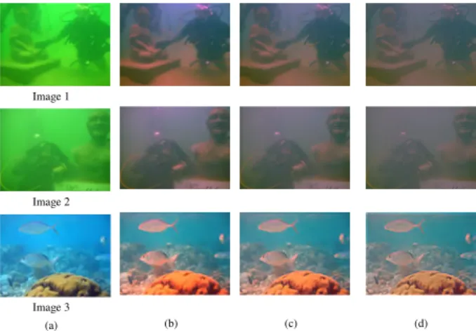
Fig. 4 (a) Source image and enhanced images that are processed with the (b) GW method, (c) AGW method whereL=10, α=0.75, and (d) AGW method whereL=10, α=0.50.
channels and ¯Rc, ¯G, ¯Bc are the global mean for each color channel of the input image of sizeM×N. In some cases, as shown in Fig. 4, by just using only GW method, not only it removes color cast but introduces some reddishness that may affect the visual aspects of the image. To reduce this reddish cast, a combination of weighted global mean and weighted local mean is used in this study. The local mean of each channel is computed using
R¯L(i,j)= 1 (2L+1)2
X
(i,j)∈WL
Rc(i,j)
G¯L(i,j)= 1 (2L+1)2
X
(i,j)∈WL
G(i,j) B¯L(i,j)= 1
(2L+1)2 X
(i,j)∈WL
Bc(i,j)
(3)
where WL is the moving local average window size for (2L+1)×(2L+1)region withLis set to 10. This calcu- lation, otherwise known as local averaging operation, where the value of each pixel is replaced by the average of all the values in the local neighborhood. The edge borders of the processing images are padded with mirror reflections of themselves.
Next, both the global and local mean values are scaled and combined as follows
R¯θ(i,j)=α·R¯c+(1−α)·R¯L(i,j) G¯θ(i,j)=α·G¯+(1−α)·G¯L(i,j) B¯θ(i,j)=α·B¯c+(1−α)·B¯L(i,j)
(4)
where 0≤α≤1 and ¯Rθ(i,j), ¯Gθ(i,j), ¯Bθ(i,j)represent the compensation mean value for each channel. Subsequently, the AGW is obtained by averaging out the compensated color channels with compensation mean value which can be ex- pressed as
Table 1 Comparative results of GW and AGW using UCIQE[32]and UIQM[33]metrics.
source GW AGW,
α=0.75 AGW, α=0.50 UCIQE
Image 1 0.392 0.489 0.472 0.457
Image 2 0.405 0.493 0.478 0.463
Image 3 0.532 0.559 0.550 0.542
UIQM
Image 1 0.363 0.659 0.639 0.620
Image 2 0.347 0.508 0.499 0.491
Image 3 0.677 0.908 0.886 0.860
R(i,ˆ j)= Rc(i,j) R¯θ(i,j)·m G(i,ˆ j)= G(i,j)
G¯θ(i,j)·m B(i,ˆ j)= Bc(i,j)
B¯θ(i,j) ·m
(5)
where
m= 1
3M N X
i∈M
X
j∈N
[ ¯Rθ(i,j)+G¯θ(i,j)+B¯θ(i,j)] (6)
3.2 Performance Analysis of GW and AGW
A qualitative comparison between the enhanced images that are processed with GW and AGW methods is shown in Fig. 4, while the quantitative evaluations using UCIQE and UIQM metric are shown in Table 1. It is noticeably seen that en- hanced images shown in second column of Fig. 4 that used GW method have more reddish casts especially on the water bubbles and background areas when compared to the en- hanced images shown in third and fourth columns of Fig. 4 that used AGW method. The underwater metrics UCIQE and UIQM gave higher scores for images in second column of Fig. 4. This is due to one of the measureable components in the UCIQE and UIQM metrics that consider the colorfulness of the bubbles and objects that may not necessarily correlate to the human visual system evaluation. For example, the bubbles should be ideally colorless and the purpose of using the local mean is to reduce this reddishness. Nevertheless, the contrast and colorfulness of the enhanced images that are processed with AGW method can be further improved by integrating the DHECI method.
3.3 Contrast Enhancement
In this paper, the DHECI method is adopted from[34]and it is applied to improve the contrast and colorfulness of the image. The DHECI method is actually an extended version of DHE[35]for a color image. Unlike grayscale images, there are some factors in color images like hue components that need to be properly taken care for enhancement. In other words, hue-preserving enhancement methods[36]–[38]are required and the color image is transformed fromRGBtoHSI color space by using the transformation formula represented in Ref.[39]. Nakai et al.[34]have defined two differential
Fig. 5 The flowchart of the computation of the DHECI method.
gray-levels histograms for color images which are Differen- tial Intensity Gray-Levels Histogram Equalization (DIHE) and Differential Saturation Gray-Levels Histogram Equal- ization (DSHE) that are applied to intensity and saturation components, respectively. The hue component remains un- changed. The flowchart of the computation of the DHECI method is shown in Fig. 5.
Let I(i,j) and S(i,j) be the intensity and saturation components of the image. The intensity component is com- puted as
I(i,j)=1
3 ·[ ˆR(i,j)+G(i,ˆ j)+B(i,ˆ j)] (7) and the differential intensity gray-levelsdI(i,j)of the image is calculated using
dI(i,j)=round(
q
dIH(i,j)2+dVI(i,j)2), where
dIH(i,j)=[I(i+1,j+1)+2·I(i+1,j)+I(i+1,j−1)]
−[I(i−1,j+1)+2·I(i−1,j)+I(i−1,j−1)]
dVI(i,j)=[I(i+1,j+1)+2·I(i,j+1)+I(i−1,j+1)]
−[I(i+1,j−1)+2·I(i,j−1)+I(i−1,j−1)]
(8)
Next, the differential intensity gray-level histogram (DIH) is computed using
hId(r)= X
(i,j)∈Dr
dI(i,j) (9)
where Dr is a region composed of pixels whose value is r that takes the values between 0 and 255. In other words, the horizontal axis of DIH is gray-levelrwhile the vertical axis is the total differential gray-levels ofI(i,j)points which meet the conditionI(i,j)=r. For example, the total sum of the computation ofhId(0)is obtained by summing the values ofdI(i,j), where(i,j)are the locations ofI(i,j)=0.
In the case of computing the saturation component, the approach is similar to the intensity component computations.
First, the saturation component of the image is computed as
S(i,j)= 1− 3
(R(i,j)+G(i,j)+B(i,j))·a
!
(10) wherea is the minimum value among R(i,j), G(i,j) and B(i,j). Similiar to the computation ofdI(i,j), the differen- tial saturation gray-levelsdS(i,j)of the image is computed using
dS(i,j)=round(
q
dSH(i,j)2+dVS(i,j)2), where
dSH(i,j)=[S(i+1,j+1)+2·S(i+1,j)+S(i+1,j−1)]
−[S(i−1,j+1)+2·S(i−1,j)+S(i−1,j−1)]
dVS(i,j)=[S(i+1,j+1)+2·S(i,j+1)+S(i−1,j+1)]
−[S(i+1,j−1)+2·S(i,j−1)+S(i−1,j−1)]
(11)
And, the computation of the differential saturation gray-level histogram (DSH) is given by
hSd(r)= X
(i,j)∈Dr
dS(i,j) (12)
where Dr is a region composed of pixels whose intensity value isr, which isI(i,j)=r. The computation ofhSd(r)is obtained in the same way as in the computation ofhdI(r).
For the case of color image, two differential gray-levels histograms, which are DIH and DSH, are then combined for both contrast and colorfulness of the image, respectively.
The combined histogram is given by
hcolord (r)=αc·hSd(r)+(1−αc)·hId(r) (13) whereαc is the scale factor in the range of 0 ≤ αc ≤ 1.
The DHECI is obtained using the following transformation function
s(r)=255·
* . . . . ,
Pr
k=0hcolord (k)
255P
k=0hcolord (k) + / / / / -
(14)
Lastly, the enhanced image RGBo(i,j) is then com- puted using
Ro(i,j)=s(R(i,ˆ j)) Go(i,j)=s(G(i,ˆ j)) Bo(i,j)=s(B(i,ˆ j))
(15)
4. Experimental Results and Discussion
In this section, we begin with the analysis of parameters se- lection for local window size (L) in AGW and scale factor alpha (αc) in DHECI. Then, the qualitative and quantitative differences between the proposed method and the state-of- the-art methods are carried out using the following four met- rics: Entropy, Patch-based Contrast Quality Index (PCQI) [40], Underwater Color Image Quality Evaluation (UCIQE)
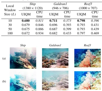
Table 2 Quantitative evaluations of UIQM scores and CPU time (in seconds) for the proposed method with varied local window size (L).
Local Window Size (L)
Ship Galdran1 Reef3
(1380×1120) (946×706) (1000×707)
UIQM CPU
time UIQM CPU
time UIQM CPU
time 10 0.680 0.811 0.711 0.373 0.798 0.396
30 0.679 0.846 0.696 0.393 0.793 0.431
50 0.675 0.886 0.687 0.399 0.793 0.439
100 0.672 0.934 0.682 0.433 0.797 0.469
Fig. 6 Visual comparison for three enhanced underwater images (Ship, Galdran1, Reef3) that are processed with the proposed method where α=0.5,L=10, (a)αc=0 and (b)αc=1 in the DHECI method.
[32], and Underwater Image Quality Measure (UIQM)[33].
Entropy is used to measure the image information content where the higher entropy values of an image indicate more information contained in that particular image. As given by Eq. (16), it is calculated as the summation of the products of the probability of outcome multiplied by the log of the inverse of the outcome probability.
Entropy=−
n
X
i=1
p(i)
log2p(i)
(16) wherenis the total number of intensity level,pirepresents the probability that the difference between two adjacent pix- els is equal toi. PCQI is a general-purpose image contrast metric that assessed the image quality of contrast changed based on an adaptive representation of local patch structure.
According to Ref.[40], they represented any image patch in a unique and adaptive way as three conceptually indepen- dent components, which areqi(x, y),qc(x, y)andqs(x, y) that refer to the mean intensity, signal strength and signal structure, respectively. It is defined as
PCQI(X,Y)= 1 M
M
X
j=1
qi(x, y)·qc(x, y)·qs(x, y) (17) where X is the original image,Y is the test image and M is the total number of patches. One significant advantage of PCQI is that when it is applied to local patches across the image, a spatially varying quality map is created, which delivers useful information about the local quality variations across space. The higher PCQI values indicate the image has better contrast. On the other hand, the UCIQE metric is designed specifically to quantify the non-uniform color
Table 3 Underwater quantitative evaluations of ENTROPY for Fig. 7.
Source [15] [19] [23] [24] [20] [31] [6] Proposed
method
Ship 7.186 7.218 6.833 7.872 7.576 7.133 7.554 7.728 7.762
Fish 6.708 7.815 6.838 6.224 7.352 6.680 7.035 7.824 7.678
Reef1 7.252 7.288 7.360 6.670 7.507 7.217 7.402 7.582 7.749
Reef2 6.729 7.502 6.494 6.141 6.780 6.706 6.707 7.582 7.145
Reef3 7.061 7.711 7.185 6.821 7.753 7.048 7.679 7.903 7.890
Ancuti1 6.926 7.153 6.909 7.918 6.817 7.359 7.667 7.852 7.847
Ancuti2 6.169 6.314 6.420 7.103 6.963 6.771 7.401 7.823 7.700
Ancuti3 6.237 6.516 6.836 7.431 6.965 6.881 7.749 7.678 7.765
Average 6.783 7.190 6.859 7.023 7.214 6.974 7.399 7.747 7.692
Table 4 Underwater quantitative evaluations of PCQI for Fig. 7.
Source [15] [19] [23] [24] [20] [31] [6] Proposed
method
Ship - 0.446 0.649 0.920 0.945 0.981 1.172 1.048 1.127
Fish - 1.135 0.863 0.835 1.156 0.980 1.117 1.164 1.260
Reef1 - 0.996 1.046 0.794 1.078 0.963 1.083 0.996 1.139
Reef2 - 1.162 0.483 0.769 0.607 0.976 1.075 1.135 1.064
Reef3 - 1.050 0.793 0.883 0.943 1.028 1.276 1.184 1.252
Ancuti1 - 0.813 0.909 0.962 1.036 0.986 1.022 1.062 1.180
Ancuti2 - 0.778 0.475 0.591 0.603 1.022 0.914 1.072 1.240
Ancuti3 - 0.961 0.973 1.021 1.129 1.003 1.207 1.143 1.269
Average - 0.918 0.774 0.847 0.937 0.992 1.108 1.101 1.191
Table 5 Underwater quantitative evaluations of UCIQE for Fig. 7.
Source [15] [19] [23] [24] [20] [31] [6] Proposed
method
Ship 0.554 0.810 0.550 0.646 0.632 0.548 0.632 0.739 0.742
Fish 0.532 0.747 0.623 0.527 0.705 0.527 0.667 0.695 0.701
Reef1 0.578 0.736 0.649 0.576 0.660 0.571 0.658 0.715 0.736
Reef2 0.645 0.709 0.659 0.633 0.718 0.622 0.711 0.710 0.730
Reef3 0.519 0.746 0.620 0.533 0.678 0.519 0.697 0.713 0.735
Ancuti1 0.425 0.458 0.499 0.641 0.499 0.457 0.594 0.699 0.741
Ancuti2 0.412 0.433 0.492 0.529 0.529 0.442 0.592 0.689 0.691
Ancuti3 0.419 0.435 0.535 0.614 0.555 0.459 0.664 0.731 0.727
Average 0.511 0.634 0.578 0.587 0.622 0.518 0.652 0.711 0.725
Table 6 Underwater quantitative evaluations of UIQM for Fig. 7.
Source [15] [19] [23] [24] [20] [31] [6] Proposed
method
Ship 0.475 0.722 0.492 0.605 0.588 0.483 0.668 0.589 0.610
Fish 0.677 0.876 0.571 0.528 0.759 0.669 0.624 0.757 0.834
Reef1 0.752 0.861 0.657 0.565 0.690 0.705 0.687 0.994 0.608
Reef2 0.854 0.805 0.653 0.671 0.757 0.807 0.781 0.914 0.856
Reef3 0.730 0.637 0.584 0.524 0.677 0.708 0.766 0.638 0.748
Ancuti1 0.348 0.519 0.383 0.458 0.407 0.591 0.507 0.601 0.640
Ancuti2 0.365 0.499 0.344 0.525 0.425 0.596 0.687 0.653 0.811
Ancuti3 0.436 0.509 0.492 0.646 0.563 0.672 0.651 0.573 0.731
Average 0.580 0.679 0.522 0.565 0.608 0.654 0.671 0.715 0.730
cast, blurring, and low-contrast of underwater images, while UIQM metric addresses three important underwater image quality criterions: colorfulness, sharpness and contrast. The UCIQE metric for an imageIin CIELAB space is defined as
UCIQE=c1×σc+c2×conl+c3×µs (18) where σc is the standard deviation of chroma, conl is the contrast of luminance and µs is the average of satu- ration, and c1,c2,c3 are weighted coefficients. For under- water monitoring and survey color images with blurring,
color cast and marine snow distortions, the coefficients are c1 = 0.4680,c2 = 0.2745,c3 = 0.2576. The UCIQE ap- proach is promising in terms of both computational effi- ciency and practical reliability for real-time applications.
Most importantly, it is a meaningful structural model to real- ize effective underwater color. The UIQM comprises three underwater image attribute measures, which are Underwa- ter Image Colorfulness Measure (UICM), Underwater Image Sharpness Measure (UISM) and Underwater Image Contrast Measure (UIConM). Each attribute is selected for evaluating one aspect of the underwater image degradation, and each
Fig. 7 Visual comparison for eight underwater images. (a) Source images and their respective en- hanced images after processing with the (b)[15]method, (c)[19]method, (d)[23]method, (e)[24]
method, (f)[20]method, (g)[31]method (h)[6]method and (i) proposed method (L=10, α=0.5 andαc=0.1). The quantitative evaluation associated with these images is provided in Tables 3–6.
presented attribute measure is inspired by the properties of HVS. Refer to Ref.[33], the overall underwater image quality measure is given by
UIQM=c1×UICM+c2×UISM+c3×UIConM (19) where the colorfulness, sharpness and contrast measures are linearly combined together.
4.1 Selection of Parameters
In this experimental study, the local average window size (L) in compensation mean of AGW is set to 10. Experiments were carried out to show the performance of using different local window size (L =[10,30,50,100]). Since the results of UCIQE and UIQM metrics follow the same trend, so only one of them have been shown. The quantitative scores of different L using UIQM as well as the CPU time (in seconds) for three images (Ship,Galdran1,Reef3) are shown in Table 2. The values in bold in the Table 2 represent better UIQM scores, while the values in italic represent shortest CPU times. The results of UIQM metric in Table 2 indicate
that the smaller values ofLwould yield better UIQM scores compared to the higher values ofL. Thus,L=10 is selected as it takes less computational time too when compared to the higher local window size.
Next, the significance ofαcin DHECI can be seen in Fig. 6. Whenαc=1, the intensity component becomes zero in Eq. (13). Hence, there is a loss of color when compared toαc =0. On the other hand, whenαc =0, the saturation component in Eq. (13) is zero, hence the brightness in the images as shown in the Fig. 6(a) is quite high. Fig. 6(a) and (b) show the effects of αc = 0 and αc = 1, respectively.
In this study, αc = 0.1 have been used. The role of the saturation is to lower the overall intensity. By increasing αc, the values of the intensity component decrease while the saturation component increase which both contributes to the enhancement of the image.
4.2 Comparative Analysis Using Qualitative and Quantita- tive Evaluation
Figure 7 presents the results obtained on underwater images
by different underwater environment approaches, which in- clude Carlevaris-Bianco et al.[15]method, Drews-Jr et al.
[19]method, Galdran et al. [23] method, Emberton et al.
[24]method, Li et al.[20]method, Ancuti et al.[31]method and Wong et al.[6]method. Tables 3, 4, 5 and 6 provide the associated quantitative evaluation using four metrics: En- tropy, PCQI, UCIQE and UIQM. In this study, there are eight images have been selected to be used for both qualitative and quantitative evaluations.
As can be seen in Fig. 7, the source underwater images consist of color cast, haze and lack of contrast. It is noticeable that the methods of Galdran et al.[23]and Ancuti et al.[31]
have consistently removed the greenish and bluish casts in the whole underwater images and recovered visibility. However, as attested by the last two columns in Fig. 7, our work in Ref.
[6]and the proposed method not only removed the undesired color cast and improved the visibility, they have increased the brightness and preserved natural appearance of the un- derwater images. Furthermore, the overall resultant images produced by proposed method showed an improvement in terms of image contrast and color. The objects or subjects in the underwater images are well-observed and leave a better impression to the viewers. This can be further validated by the quantitative assessments where our proposed method having averagely higher values of the PCQI, UCIQE and UIQM metrics. For the methods of Carlevaris-Bianco et al.[15], Drews-Jr et al.[19], Emberton et al. [24]and Li et al. [20], some greenish and bluish casts still remain in their enhanced images as their methods are more focused on dehazing in underwater scenes.
5. Conclusion
In this paper, a structure consisting of AGW and DHECI methods is proposed to remove the color cast as well as to enhance the contrast and colorfulness in underwater images.
AGW method is an adaptive version of GW where apart from computing the global mean, the local mean of each channel of an image is taken into consideration and both are weighted before combining them together. However, before the color cast removal AGW method is applied, the red and blue chan- nels of underwater images are first being compensated due to the very small mean value that caused severe red artifacts occurred. Thereafter, the DHECI method is employed to in- crease the contrast and colorfulness of the image. The results of the proposed method are compared with seven state-of- the-art methods using qualitative and quantitative measures.
The proposed method has increased the visibility of under- water images and in most cases produces better quantitative scores when compared to the seven state-of-the-art methods.
References
[1] J. Yuh and M. West, “Underwater robotics,” Adv. Robot., vol.15, no.5, pp.609–639, Jan. 2001.
[2] S.Q. Duntley, “Light in the sea,” J. Opt. Soc. Am., vol.53, no.2, pp.214–233, Feb. 1963.
[3] E. Trucco and A. Olmos-Antillon, “Self-tuning underwater image
restoration,” IEEE J. Oceanic Eng., vol.31, no.2, pp.511–519, April 2006.
[4] R. Schettini and S. Corchs, “Underwater image processing: State of the art of restoration and image enhancement methods,” EURASIP J. Adv. Signal Process., vol.2010, no.1, p.746052, Dec. 2010.
[5] Viki, “Avoiding backscatter in underwater photography,” Scubafish News, http://news.scubafish.com/latest-news/avoiding-backscatter- in-underwater-photography/, accessed June 2012.
[6] S.L. Wong, R. Paramesran, and A. Taguchi, “Underwater image enhancement by adaptive gray world and differential gray-levels his- togram equalization,” Advances in Electrical and Computer Engi- neering, vol.18, no.2, pp.109–116, 2018.
[7] X. Liu, G. Zhong, C. Liu, and J. Dong, “Underwater image colour constancy based on DSNMF,” IET Image Processing, vol.11, no.1, pp.38–43, Jan. 2017.
[8] Y.T. Peng and P.C. Cosman, “Underwater image restoration based on image blurriness and light absorption,” IEEE Trans. Image Process., vol.26, no.4, pp.1579–1594, April 2017.
[9] H. Lu, Y. Li, X. Xu, J. Li, Z. Liu, X. Li, J. Yang, and S. Serikawa, “Un- derwater image enhancement method using weighted guided trigono- metric filtering and artificial light correction,” J. Vis. Commun. Im- age R., vol.38, pp.504–516, 2016.
[10] J. Ao and C. Ma, “Adaptive stretching method for underwater image color correction,” Int. J. Patt. Recogn. Artif. Intell., vol.32, no.02, p.1854001, Feb. 2018.
[11] G. Hou, Z. Pan, B. Huang, G. Wang, and X. Luan, “Hue preserving- based approach for underwater colour image enhancement,” IET Image Process., vol.12, no.2, pp.292–298, 2018.
[12] R.T. Tan, “Visibility in bad weather from a single image,” 2008 IEEE Conference on Computer Vision and Pattern Recognition, pp.1–8, IEEE, June 2008.
[13] R. Fattal, “Single image dehazing,” ACM Trans. Graph., vol.27, no.3, p.1, Aug. 2008.
[14] R. Fattal, “Dehazing using color-lines,” ACM Trans. Graph., vol.34, no.1, pp.1–14, Dec. 2014.
[15] N. Carlevaris-Bianco, A. Mohan, and R.M. Eustice, “Initial results in underwater single image dehazing,” Oceans 2010 MTS/IEEE SEAT- TLE, pp.1–8, IEEE, Sept. 2010.
[16] J.Y. Chiang and Y.C. Chen, “Underwater image enhancement by wavelength compensation and dehazing,” IEEE Trans. Image Pro- cess., vol.21, no.4, pp.1756–1769, April 2012.
[17] K. He, J. Sun, and X. Tang, “Single image haze removal using dark channel prior,” 2009 IEEE Conference on Computer Vision and Pattern Recognition, pp.1956–1963, IEEE, June 2009.
[18] K. He, J. Sun, and X. Tang, “Single image haze removal using dark channel prior,” IEEE Trans. Pattern Anal. Mach. Intell., vol.33, no.12, pp.2341–2353, Aug. 2011.
[19] P. Drews, Jr, E. do Nascimento, F. Moraes, S. Botelho, and M. Cam- pos, “Transmission estimation in underwater single images,” 2013 IEEE International Conference on Computer Vision Workshops, pp.825–830, IEEE, Dec. 2013.
[20] C. Li, J. Guo, S. Chen, Y. Tang, Y. Pang, and J. Wang, “Underwater image restoration based on minimum information loss principle and optical properties of underwater imaging,” 2016 IEEE International Conference on Image Processing (ICIP), pp.1993–1997, IEEE, Sept.
2016.
[21] C. Li, J. Guo, R. Cong, Y. Pang, and B. Wang, “Underwater im- age enhancement by dehazing with minimum information loss and histogram distribution prior,” IEEE Trans. Image Process., vol.25, no.12, pp.5664–5677, Dec. 2016.
[22] H. Lu, Y. Li, S. Nakashima, and S. Serikawa, “Turbidity underwater image restoration using spectral properties and light compensation,”
IEICE Trans. Inf. & Syst., vol.E99-D, no.1, pp.219–227, Jan. 2016.
[23] A. Galdran, D. Pardo, A. Picón, and A. Alvarez-Gila, “Automatic red-channel underwater image restoration,” J. Vis. Commun. Image R., vol.26, pp.132–145, Jan. 2015.
[24] S. Emberton, L. Chittka, and A. Cavallaro, “Hierarchical rank-based
veiling light estimation for underwater dehazing,” Proc. British Ma- chine Vision Conference 2015, pp.125.1–125.12, British Machine Vision Association, 2015.
[25] G. Buchsbaum, “A spatial processor model for object colour percep- tion,” J. Franklin Institute, vol.310, no.1, pp.1–26, 1980.
[26] W.J. Kyung, D.C. Kim, H.G. Ha, and Y.H. Ha, “Color enhancement for faded images based on multi-scale gray world algorithm,” 2012 IEEE 16th International Symposium on Consumer Electronics, pp.1–
4, IEEE, June 2012.
[27] N. Kwok, D. Wang, X. Jia, S. Chen, G. Fang, and Q. Ha, “Gray world based color correction and intensity preservation for image enhancement,” 2011 4th International Congress on Image and Signal Processing, pp.994–998, IEEE, Oct. 2011.
[28] G. Bianco, M. Muzzupappa, F. Bruno, R. Garcia, and L. Neumann,
“A new color correction method for underwater imaging,” ISPRS - International Archives of the Photogrammetry, Remote Sensing and Spatial Information Sciences, vol.XL-5/W5, pp.25–32, 2015.
[29] D. Park, D.K. Han, and H. Ko, “Enhancing underwater color images via optical imaging model and non-local means denoising,” IEICE Trans. Inf. & Syst., vol.E100-D, no.7, pp.1475–1483, July 2017.
[30] C. Ancuti, C.O. Ancuti, T. Haber, and P. Bekaert, “Enhancing un- derwater images and videos by fusion,” 2012 IEEE Conference on Computer Vision and Pattern Recognition, pp.81–88, IEEE, June 2012.
[31] C.O. Ancuti, C. Ancuti, C. De Vleeschouwer, and P. Bekaert, “Color balance and fusion for underwater image enhancement,” IEEE Trans.
Image Process., vol.27, no.1, pp.379–393, Jan. 2018.
[32] M. Yang and A. Sowmya, “An underwater color image quality eval- uation metric,” IEEE Trans. Image Process., vol.24, no.12, pp.6062–
6071, Dec. 2015.
[33] K. Panetta, C. Gao, and S. Agaian, “Human-visual-system-inspired underwater image quality measures,” IEEE J. Ocean. Eng., vol.41, no.3, pp.541–551, 2016.
[34] K. Nakai, Y. Hoshi, and A. Taguchi, “Color image contrast enhace- ment method based on differential intensity/saturation gray-levels histograms,” 2013 International Symposium on Intelligent Signal Processing and Communication Systems, pp.445–449, 2013.
[35] K. Murahira and A. Taguchi, “A novel contrast enhancement method using differential gray-levels histogram,” 2011 International Sympo- sium on Intelligent Signal Processing and Communications Systems (ISPACS), pp.1–5, IEEE, Dec. 2011.
[36] A. Taguchi and Y. Hoshi, “Color image enhancement in HSI color space without gamut problem,” IEICE Trans. Fundamentals, vol.E98-A, no.2, pp.792–795, Feb. 2015.
[37] M. Kamiyama and A. Taguchi, “HSI color space with same gamut of RGB color space,” IEICE Trans. Fundamentals, vol.E100-A, no.1, pp.341–344, Jan. 2017.
[38] M. Kamiyama and A. Taguchi, “Hue-preserving color image pro- cessing with a high arbitrariness in RGB color space,” IEICE Trans.
Fundamentals, vol.E100-A, no.11, pp.2256–2265, Nov. 2017.
[39] R.C. Gonzalez and R.E. Woods, Digital Image Processing, 3rd ed., Prentice Hall, New Jersey, 2008.
[40] S. Wang, K. Ma, H. Yeganeh, Z. Wang, and W. Lin, “A patch- structure representation method for quality assessment of con- trast changed images,” IEEE Signal Process. Lett., vol.22, no.12, pp.2387–2390, Dec. 2015.
Siaw-Lang Wong received both B.CompSc and M.Sc degrees in computer science from Uni- versiti Teknikal Malaysia Melaka, Malaysia in 2009 and 2011 respectively. She has joined Uni- versiti Tunku Abdul Rahman, Malaysia as a lec- turer in 2011 to 2013. She is currently pursuing her Ph.D in Department of Electrical Engineer- ing at University of Malaya, Malaysia. Her re- search interests include image compression, im- age enhancement and image restoration.
Raveendran Paramesran received the B.Sc and M.Sc degrees in electrical engineering from South Dakota State University, Brookings, South Dakota, USA in 1984 and 1985 respectively. He was a systems designer with Daktronics, U.S.A before joining the Department of Electrical Engi- neering at University of Malaya, Kuala Lumpur, as a lecturer in 1986. In 1992, he received a Ron- paku scholarship from Japan to pursue Doctorate in Engineering, which he completed in 1994 at University of Tokushima, Japan. He was pro- moted to Associate Professor in 1995 and was promoted to Professor in 2003. His research areas include image and video analysis, formulation of new image descriptors for image analysis, fast computation of orthogonal moments, analysis of EEG signals, and data modeling of substance concen- tration acquired from non-invasive methods. His contributions can be seen in the form of journal publications, conference proceedings, chapters in books and an international patent to predict blood glucose levels using non- parametric model. He has successfully supervised to completion 18 Ph.D students and 13 students in M.Eng.Sc (Masters by research). He is currently a Senior IEEE member and also a member of the Signal Processing Society.
Ibuki Yoshida received the B.E. degree in Computer Science from Tokyo City University in 2018. He has enrolled in graduate school of Tokyo City University. His research interest in color image processing. He is a student member of IEEE.
Akira Taguchi received B.E., M.E. and Dr. Eng. Degrees in electrical engineering from Keio University, Yokohama, in 1984, 1986 and 1989 respectively. In 1989, he joined Musashi Institute of Technology (renamed Tokyo City University). He is currently a Professor at the Department of Computer Science, Tokyo City University. From 1993 to 1994 he spent one year at the Signal Processing Laboratory, Tam- pere University of Technology, Finland as a Vis- iting Researcher. His research interests are the areas of digital image processing including nonlinear signal processing and color image processing. He served as the editor of IEICE Trans. on Fun- damentals from 2001 to 2003. He was appointed as the General Chair for ISPACS 2013 (IEEE). He is a member of the DSP Technical Committee of IEEE Circuits and System Society and he is a chair of the steering com- mittee of ISPACS. He is a senior member of IEEE and a fellow of IEICE.
Currently, he is the President-Elect of Engineering Sciences Society, IEICE.
![Fig. 1 Absorption of light by water. Image courtesy of Duntley [2].](https://thumb-ap.123doks.com/thumbv2/123deta/5634521.1501536/1.892.551.729.308.461/fig-absorption-light-water-image-courtesy-duntley.webp)
![Table 1 Comparative results of GW and AGW using UCIQE [32] and UIQM [33] metrics. source GW AGW, α = 0.75 AGW,α= 0.50 UCIQE Image 1 0.392 0.489 0.472 0.457Image 20.4050.4930.4780.463 Image 3 0.532 0.559 0.550 0.542 UIQM Image 1 0.363 0.659 0.639 0.620Image](https://thumb-ap.123doks.com/thumbv2/123deta/5634521.1501536/4.892.544.737.120.358/table-comparative-results-uciqe-metrics-source-uciqe-image.webp)
![Table 3 Underwater quantitative evaluations of ENTROPY for Fig. 7. Source [15] [19] [23] [24] [20] [31] [6] Proposed method Ship 7.186 7.218 6.833 7.872 7.576 7.133 7.554 7.728 7.762 Fish 6.708 7.815 6.838 6.224 7.352 6.680 7.035 7.824 7.678 Reef1 7.252 7.](https://thumb-ap.123doks.com/thumbv2/123deta/5634521.1501536/6.892.127.769.136.299/table-underwater-quantitative-evaluations-entropy-source-proposed-method.webp)
![Fig. 7 Visual comparison for eight underwater images. (a) Source images and their respective en- en-hanced images after processing with the (b) [15] method, (c) [19] method, (d) [23] method, (e) [24]](https://thumb-ap.123doks.com/thumbv2/123deta/5634521.1501536/7.892.73.823.119.652/visual-comparison-underwater-images-source-images-respective-processing.webp)
