Kobayashi Potential in Electromagnetism

INVITED PAPER

Kobayashi Potential in Electromagnetism

Kohei HONGO^†,Nonmember andHirohide SERIZAWA^††a),Member

SUMMARY The Kobayashi potential in electromagnetic theory is re- viewed. As an illustration we consider two problems, diffraction of plane wave by disk and rectangular plate of perfect conductor. Some numeri- cal results are compared with approximated and experimental results when they are available to verify the validity of the present method. We think the present method can be used as reference solutions of the related problems.

key words: Kobayashi potential, mixed boundary value problem, diffrac- tion and scattering, edge condition

1. Introduction

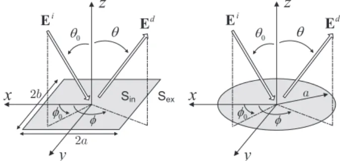
The name of the Kobayashi potential (KP) was given by I. Sneddon in his book “Mixed Boundary Value Problems in Potential Theory” [1] for the paper [2] published by Kobayashi in 1931. This paper treated the potential prob- lems associated with single disk or two disks. He assumed a potential function so that the function becomes in the form of Weber-Schafheitlin’s discontinuous integrals in the plane z = 0 where the circular plate is located. This makes the function satisfy a part of the required boundary conditions like the eigen function expansion methods in circular cylin- der and sphere scattering problems. The potential functions in static problems were extended to dynamic wave problems by Yukiti (Yukichi) Nomura and his associates. Their note- worthy work is on the paper of the diffraction of electromag- netic wave by a ribbon and a disk of perfect conductor (with Shigetoshi Katsura) [3]. Electromagnetic scattering prob- lems using the Kobayashi potential have been studied by K. Hongo and his students [4], [5]. In this paper we intro- duce an excellent technique developed in Japan since very few researchers may be familiar to this method. To deepen the understanding we show two problems as an illustration, the first is the scattering by a rectangular plate and the sec- ond one is by a disk (see Fig. 1).

The reference solution for scattering by rectangular plate is very few except the moment method solution. And this method serves its aims. Also this subject has some in- teresting problem, for example, singularity at the vertex, nu- merical solutions of the grazing incidence case, and so on.

In this paper we present rigorous formulation of this prob- lem by using the KP method. Two components of the vector

Manuscript received April 22, 2011.

Manuscript revised July 27, 2011.

†No affiliation.

††The author is with the Department of Control and Computer Engineering, Numazu National College of Technology, Numazu- shi, 410-8501 Japan.

a) E-mail: [email protected] DOI: 10.1587/transele.E95.C.3

Fig. 1 Scattering of an electromagnetic plane wave by a rectangular plate and by a circular disk. (θ0, φ0) denote the angles of incidence.

potential are expressed in terms of two dimensional Fourier sine and cosine transform. We use the discontinuous proper- ties of the Weber-Schafheitlin integrals so that the required boundary conditions at the exterior to the plate or hole in the plane where it is located. By using the concept of the projec- tion for the remaining condition on the plate, the solution is reduced to matrix equations. The matrix elements are given by double infinite integrals with rather slow convergence.

We have developed a method of computation that enables one to get precise results. The expressions thus derived have properties similar to those for eigen function solutions for a circular cylinder and a sphere.

Diffraction of EM wave by a circular hole is classical problem and exact solutions exist. Meixner formulated the field in terms of Spheroidal functions and Andrejewsky [6]

gave some numerical results. Katsura and Nomura solved the same problem by using the Weber-Schafheitlin’s inte- gral [3]. The present formulation belongs to the similar cat- egory with the work of Katsura and Nomura, but there are also some differences. Theoretically, diffracted field can be expressed by two scalar wave functions [7]. The works [3]

and [6] used three components which are related by impos- ing edge conditions. In this paper we show that the field can be derived from two components of the vector potential functions and the functions themselves satisfy the edge con- dition [8]. Therefore the philosophy of the formulation is very simple. The procedure of the formulation is as follows.

The two components of the vector potential are expanded in the form of Fourier Hankel transform [9]. By imposing the required boundary conditions dual integral equations are derived. These equations are transformed into matrix equa- tions by applying the properties of Weber-Schafheitlin’s in- tegral and projection. Matrix elements may be evaluated in Copyright c2012 The Institute of Electronics, Information and Communication Engineers

a closed form and computed rather easily. Computed results are compared with asymptotic solutions and experimental results. Agreement among them is fairly well.

2. Diffraction of Plane EM Waves by a Rectangular Plate[4], [5]

In this chapter we present how to formulate the electromag- netic plane wave diffracted by a rectangular plate or hole (hereafter we treat only plate problem). The incident wave is given by

Eⁱ =(E2iθ+E1iφ) exp[jkΦⁱ(r)] (1a) Hⁱ =Y0(−E2iφ+E1iθ) exp[jkΦⁱ(r)] (1b) and the magnetic vector potentialA^sof the scattered wave, which is used instead of the electromagnetic field for the convenience of later analysis, is given by

A^s_x A^s_y

= μ₀Y0a _∞

0

_∞

0

f_cc^±(α, β) g^±_cc(α, β)

cosαξcosβη +

f_cs^±(α, β) g^±_cs(α, β)

cosαξsinβη+

f_sc^±(α, β) g^±_sc(α, β)

sinαξ

×cosβη+

f_ss^±(α, β) g^±_ss(α, β)

sinαξsinβη

×exp

∓ζ(α, β)za

dαdβ (z≷0) (2) wheref(α, β) andg(α, β) are unknown functions determined later. The symbols used in (1) and (2) are defined by

iθ=cosθ₀cosφ₀ix+cosθ₀sinφ₀iy−sinθ₀iz,

iφ=−sinφ₀ix+cosφ₀iy (3a) Φⁱ(r)

Φ^r(r)

=xsinθ₀cosφ₀+ysinθ₀sinφ₀±zcosθ₀ (3b) ζ(α, β)= α²+p²β²−κ², ξ= x

a, η= y b, za= z

a, p=a b

=1 q

, κ=ka, Y0= ₀

μ₀. (3c) In this analysis, harmonic time dependence exp(jωt) is as- sumed and omitted in equations. Imposing the required boundary conditions:H_x^t andH^t_yare continuous for (x, y)∈ Sex andE^t_x =0 andE^t_y =0 on (x, y) ∈ Sin, we derive the dual integral equations. Equations for the continuities of magnetic field components can be solved by using the dis- continuous properties of the Weber-Schafheitlin’s integrals [10, p.99] and the results are given by

fcc(α, β) =^∞

m=0

∞ n=0

1

αζ(α, β)A^(x)_mnJ2m+1(α)J_2n(β) (4a) g_cc(α, β) =^∞

m=0

∞ n=0

1

βζ(α, β)A^(y)mnJ_2m(α)J_2n+1(β). (4b) Similar relations can be derived for other components. The solutions for the electric field components are obtained by applying the projection and we have matrix equations for

the expansion coefficients

KA(2m+1,2n,2s+1,2t) pG(2m+1,2n+2,2s+1,2t) qG(2m+1,2n,2s+1,2t+2) KB(2m+1,2n+2,2s+1,2t+2)

× A^(x)mn

D^(y)mn

=

−jΛ2s+1(κsinθ₀cosφ₀)J2t(κsinθ₀sinφ₀)Πx

jq²J2s+1(κsinθ₀cosφ₀)Λ2t+2(κsinθ₀sinφ₀)Πy

(5a)

KA(2m+1,2n+1,2s+1,2t+1) −pG(2m+1,2n+1,2s+1,2t+1)

−qG(2m+1,2n+1,2s+1,2t+1) KB(2m+1,2n+1,2s+1,2t+1)

× B^(x)mn

C^(y)mn

=

Λ2s+1(κsinθ₀cosφ₀)J2t+1(κsinθ₀sinφ₀)Πx

q²J_2s+1(κsinθ₀cosφ₀)Λ2t+1(κsinθ₀sinφ₀)Πy

(5b)

KA(2m+2,2n,2s+2,2t) −pG(2m,2n+2,2s+2,2t)

−qG(2m+2,2n,2s,2t+2) KB(2m,2n+2,2s,2t+2)

× C^(x)mn

B^(y)mn

=

Λ2s+2(κsinθ₀cosφ₀)J2t(κsinθ₀sinφ₀)Πx

q²J2s(κsinθ₀cosφ₀)Λ2t+2(κsinθ₀sinφ₀)Πy

(5c)

KA(2m+2,2n+1,2s+2,2t+1) pG(2m,2n+1,2s+2,2t+1) qG(2m+2,2n+1,2s,2t+1) KB(2m,2n+1,2s,2t+1)

× D^(x)mn

A^(y)mn

=

jΛ2s+2(κsinθ₀cosφ₀)J2t+1(κsinθ₀sinφ₀)Πx

−jq²J_2s(κsinθ₀cosφ₀)Λ2t+2(κsinθ₀sinφ₀)Πy

(5d) whereΠxandΠyare the amplitude of the incident wave. In the above equations the matrix elements are defined by

KA(m,n, μ, ν)= _∞

0

_∞

0

κ²−α² α²+p²β²−κ²

Jm(α)Jμ(α) α²

×Jn(β)Jν(β)dαdβ (6a) KB(m,n, μ, ν)=

_∞

0

_∞

0

q²κ²−β²

α²+p²β²−κ²Jm(α)J_μ(α)

×Jn(β)Jν(β)

β² dαdβ (6b)

G(m,n, μ, ν)= _∞

0

_∞

0

α²+p²β²−κ²₋¹₂

Jm(α)J_μ(α)

×Jn(β)Jν(β)dαdβ (6c) Λν(x)= Jν(x)

x . (6d)

Thus the problem is reduced to matrix equations, and they can be solved in a standard manner. Once the expan- sion coefficients are obtained, the far field, current den- sity, and other physical quantities can be obtained. The far field expression is derived by applying the stationary phase method of integration. It is found that the expression of the components of the current density is represented in terms of the Chebyshev polynomials of the first and sec- ond kind (see [4], [5]). And it is found that Jx is pro- portional to (1−ξ²)¹²(1−η²)⁻¹² and, Jy is proportional to (1−ξ²)⁻¹²(1−η²)¹². These are consistent with the required edge conditions for the field components. It is considered that the singularity at the vertex is higher than the straight

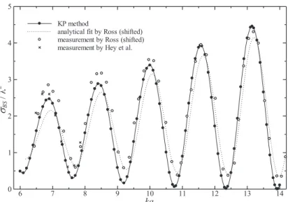
Fig. 2 Radar cross section as function of plate’s one side sizeka(kb=2π,φ0=0^◦). Ross’s data are shifted to right direction to consider plate thickness.

edge, but it is not actually correct and the singularity be- comes indefinite. It depends on how to approach to the ver- tex. As a numerical result we present here RCS of the rect- angular plate of width 2λ (kb = 2π) as a function of the normalized half-lengthka at glancing incidence since this problem has only approximate and experiment results. It is shown in Fig. 2. The experiment was done by Hey and Se- nior [11] and Ross [12]. In Fig. 2, the Ross’s data (dotted line and open circles) are shifted for the thickness.

3. Diffraction of Electromagnetic Wave by a Circular Disk[8]

This problem was studied by Meixner and Andrejewski (Spheroidal function), and Nomura and Katsura (Weber Schafheitlin’s integral) [3] as reproduced in the handbook by Bowman et al. [13] Scattered field can be expressed in terms of two scalar wave functions, but the authors cited above use three scalar wave functions since two functions lead to electromagnetic field with higher singularities. In this paper we show that the field can be derived from two scalar wave functions and these functions satisfy the required boundary conditions and edge conditions [8]. The incident wave is same as that given in (1) and the magnetic and electric vec- tor potentials of the scattered field are given by

A_z^s(ρ, φ,z) F_z^s(ρ, φ,z)

=

±μ₀aκY_{0 0}a

_∞

m=0

_∞

0

fcm(ξ) gcm(ξ)

cosmφ + fsm(ξ)

gsm(ξ)

sinmφ

Jm(ρaξ)

×exp[∓ ξ²−κ²za]ξ⁻¹dξ (7) where the upper and lower signs refer to the regionz > 0 andz < 0, respectively, andρa = ρ/a and za = z/a are the normalized variables with respect to the radiusaof the

disk (κ = kais the normalized radius). In the above equa- tions f(ξ) andg(ξ) are the unknown spectrum functions and they are to be determined so that they satisfy all the required boundary conditions. First we consider the surface fields at the planez = 0 to derive the dual integral equations asso- ciated with them. By using the relation between the vector potentials and the electromagnetic field, the tangential com- ponents of the electric field and the current density on the disk become

E_ρ^d(ρ, φ,0) E_φ^d(ρ, φ,0)

=^∞

m=0

Eρc,m(ρa) Eφc,m(ρ_a)

cosmφ+

Eρs,m(ρa) Eφs,m(ρ_a)

sinmφ

(8a) Kρ(ρ, φ) Kφ(ρ, φ)

=

−2H^d_φ(ρ, φ,0) 2H^d_ρ(ρ, φ,0)

=^∞

m=0

Kρc,m(ρa) Kφc,m(ρa)

cosmφ +

Kρs,m(ρ_a) Kφs,m(ρa)

sinmφ

(8b) where the Fourier components are written in the form of the vector Hankel transform given below:

Eρc,m(ρ_a) Eφs,m(ρa)

= _∞

0

H⁻(ξρa)j

ξ²−κ²fcm(ξ)ξ⁻¹ gsm(ξ)ξ⁻¹

ξdξ (9a) Eρs,m(ρa)

Eφc,m(ρa)

= _∞

0

H⁺(ξρa)j

ξ²−κ²fsm(ξ)ξ⁻¹ gcm(ξ)ξ⁻¹

ξdξ (9b) Kρc,m(ρa)

Kφs,m(ρa)

=2Y0

_∞

0

H⁻(ξρa) κfcm(ξ)ξ⁻¹ j

ξ²−κ²g_sm(ξ)(κξ)⁻¹

ξdξ

= _∞

0

H⁻(ξρa)Kρc,m(ξ) Kφs,m(ξ)

ξdξ (9c)

Kρs,m(ρa) Kφc,m(ρa)

=2Y0

_∞

0

H⁺(ξρa) κfsm(ξ)ξ⁻¹ j

ξ²−κ²g_cm(ξ)(κξ)⁻¹

ξdξ

= _∞

0

H⁺(ξρa)Kρs,m(ξ) Kφc,m(ξ)

ξdξ. (9d)

In the above equations the kernel matrices

H⁺(ξρa) and

H⁻(ξρa)

are given by H^±(ξρ_a)

=

⎡⎢⎢⎢⎢⎢

⎢⎢⎢⎢⎣ J_m(ξρ_a) ± m ξρa

Jm(ξρ_a)

± m ξρa

Jm(ξρ_a) J_m(ξρ_a)

⎤⎥⎥⎥⎥⎥

⎥⎥⎥⎥⎦. (10) The spectrum functions given in the right hand sides of (9) are obtained by applying the vector Hankel transform pair defined by [9]. The required boundary conditions state that the current densities on the planez = 0 are zero for ρa ≥ 1 and the tangential components of the total electric field vanish on the disk. These are written as

_∞

0

H⁻(ξρ_a)Kρc,m(ξ) Kφs,m(ξ)

ξdξ=0, _∞

0

H⁺(ξρa)Kρs,m(ξ) Kφc,m(ξ)

ξdξ=0, ρa≥1 (11) E_ρc,m^t (ρa)

E_φs,m^t (ρa)

= _∞

0

H⁻(ξρa)j

ξ²−κ²fcm(ξ)ξ⁻¹ g_sm(ξ)ξ⁻¹

ξdξ +

Eⁱ_ρc,m(ρa) E_φs,mⁱ (ρa)

=0, ρa≤1 (12a) E^t_ρs,m(ρa)

E_φc,m^t (ρ_a)

= _∞

0

H⁺(ξρ_a)j

ξ²−κ²fsm(ξ)ξ⁻¹ gcm(ξ)ξ⁻¹

ξdξ +

Eⁱ_ρs,m(ρa) E_φc,mⁱ (ρa)

=0, ρa≤1 (12b) where the superscript “t” refers to the total field. In the above equations Eⁱ_ρc,m and E_ρs,mⁱ denote the cosmφ and sinmφparts of the incident waveEⁱ_ρ, respectively, and same is true for Eⁱ_φc,m and E_φs,mⁱ . Equations (11) and (12) are the dual integral equations to determine the spectrum func- tions fm(ξ)sandgm(ξ)s. To solve (11) we expandK(ρa) in terms of the functions which satisfy Maxwell’s equations and the edge conditions. These functions can be found by taking into account the discontinuity property of the Weber- Schafheitlin integrals. Once the expressions forK(ρa) are established, the corresponding spectrum functions can be derived by applying the vector Hankel transform. It is noted that (Kρ,Kφ) satisfy the vector Helmholtz equation

∇²K+k²K = 0 in circular cylindrical coordinates on the plane z = 0 since K andH are related by K = n ×H on the plane. Furthermore (Kρ,Kφ) have the properties Kρ ∼ (1−ρ²_a)¹² andKφ ∼ (1−ρ²_a)⁻¹² near the edge of the disk. By taking into these facts, we setKρc,m(ρa)∼Kφs,m(ρa) defined in (9c) and (9d)

Kρc,m(ρa)=^∞

n=0

AmnF⁻_mn(ρa)−BmnG⁺_mn(ρa) ,

Kρs,m(ρ_a)=^∞

n=0

CmnF_mn⁻ (ρ_a)+DmnG⁺_mn(ρ_a) ,

Kφs,m(ρa)=^∞

n=0

−AmnF⁺_mn(ρa)+BmnG⁻_mn(ρa) ,

Kφc,m(ρa)=^∞

n=0

CmnF_mn⁺ (ρa)+DmnG⁻_mn(ρa)

(13) where

F^±_mn(ρa)= _∞

0

J_|m−1|(ηρa)J_|m−1|+2n+¹

2(η)

±Jm+1(ηρa)J_m+2n+³

2(η)

η¹²dη (14a) F⁺_0n(ρa)=2

_∞

0

J₁(ηρa)J_2n+³

2(η)η¹²dη (14b) G^±_mn(ρa)=

_∞

0

J_|m−1|(ηρa)J_|m−1|+2n+³

2(η)

±Jm+1(ηρa)J_m+2n+⁵

2(η)

η⁻¹²dη (14c) G⁺_0n(ρa)=2

_∞

0

J1(ηρa)J_2n+⁵

2(η)η⁻¹²dη. (14d) These integrals are of the form of the discontinuous Weber- Schafheitlin’s integral and they can be performed analyti- cally and expressed in terms of the hypergeometric func- tions. It may readily be verified thatF^±_mn(ρa)=G^±_mn(ρa)=0 forρa ≥1, andF_mn⁺ (ρa)∼(1−ρ²_a)⁻¹²,F_mn⁻ (ρa)∼(1−ρ²_a)¹², G⁺_mn(ρa)∼(1−ρ²_a)¹², andG⁻_mn(ρa)∼(1−ρ²_a)³² near the edge ρ_a1. Thus the expressions (14) satisfy one part of the dual integral equations (11) with the unknown expansion coeffi- cients Amn ∼ Dmn. To derive the spectrum functions f(ξ) andg(ξ) of the vector potentials we first determine the spec- trum functions of the current densities, since they are related each other. These are obtained by applying the vector Han- kel transform. We see from (9c) and (9d) the spectral func- tions fcm(ξ) ∼g_sm(ξ) are represented in terms of Kρc(ξ)∼ Kφsc(ξ). Thus the solutions of (11) are established. The next problem is to solve (12) and it is done by using the projec- tion. As a set of functions we choose Jacobi’s polynomials having similar form as (14). The result is given in the form of matrix equation. It is given below:

∞ n=0

⎡⎢⎢⎢⎢⎢

⎣Amn

⎛⎜⎜⎜⎜⎜

⎝Zmp,n^(1,1)

Z_mp,n^(2,1)

⎞⎟⎟⎟⎟⎟

⎠−Bmn

⎛⎜⎜⎜⎜⎜

⎝Z^(1,2)mp,n

Z^(2,2)_mp,n

⎞⎟⎟⎟⎟⎟

⎠

⎤⎥⎥⎥⎥⎥

⎦=

⎛⎜⎜⎜⎜⎜

⎝Hm,p⁽¹⁾

H_m,p⁽²⁾

⎞⎟⎟⎟⎟⎟

⎠,

m=1,2,3,· · ·, p=0,1,2,3,· · · (15a) ∞

n=0

B_0nZ_0p,n^(1,2)=H⁽¹⁾_0,p, p=0,1,2,3,· · ·. (15b) Equations forCmnandDmnare same except the right hand sides.

Z_mp,n^(1,1)=2(m+2n+¹₂) κ

α^m_pK^m_pn

1 2,1

2

−(α^m_p +3)

×K^m_pn 5

2,1 2

−κm(2α^m_p +3)

G^m_2,pn 3

2,1 2

−G^m2,pn

3 2,3

2

(16a) Z_mp,n^(1,2)=1

κ

α^m_p

K^m_pn 1

2,1 2

−K^m_pn 1

2,5 2

−(α^m_p +3)

×

K^m_pn 5

2,1 2

−(α^m_p +3)K^m_pn 5

2,5 2

−κm

G^m_2,pn 1

2,1 2

+G2,pn

5 2,1

2

+G^m2,pn

1 2,5

2

+G^m_2,pn 5

2,5 2

(16b)

Z^(2,1)_mp,n=4m(m+2n+¹₂)(m+2p+¹₂)

κ K^m_pn

1 2,1

2

−κ

α^m_p

G^m_pn

−1 2,−1

2

−G^m_pn

−1 2,3

2

−(α^mp +1)

G^m_pn 3

2,−1 2

−G^m_pn 3

2,3 2

(16c)

Z^(2,2)_mp,n=2m(m+2p+¹₂) κ

K^m_pn

1 2,1

2

−K^m_pn 1

2,5 2

−2κ

m+2n+3

2 α^m_pG^m_2,pn

−1 2,3

2

−(α^mp +1)G^m_2,pn 3

2,3 2

(16d) Z_0p,n^(1,2)=1

κ

−pK⁰pn

1 2,5

2

+(p+1.5)K⁰_pn 5

2,5 2

(16e)

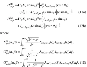
Fig. 3 Transmission coefficient of the circular aperture and RCS of the corresponding disk.

H_m,p⁽¹⁾ =4Y0E2cosθ₀j^m

α^m_pJ_m+2p+¹

2(κsinθ₀)

−(αm^p +3)J_m+2p+⁵

2(κsinθ₀)

(κsinθ₀)⁻³² (17a) H_m,p⁽²⁾ =4Y0E₂cosθ₀j^mm

J_m+2p−¹

2(κsinθ₀) +Jm+2p+³₂(κsinθ₀)

(κsinθ₀)⁻¹² (17b) where

K^mpn(α, β)= _∞

0

ξ²−κ²

ξ² Jm+2p+α(ξ)Jm+2n+β(ξ)dξ, G^m_pn(α, β)=

_∞

0

1

ξ²−κ²Jm+2p+α(ξ)Jm+2n+β(ξ)dξ, G^m_2,pn(α, β)=

_∞

0

1 ξ²

ξ²−κ²Jm+2p+α(ξ)Jm+2n+β(ξ)dξ.(18) The infinite integrals (18) may be transformed into series expansion (see [8]). We computed the transmission coeffi- cient “t” for the normal and oblique incidences for the range 0 < κ(=ka)≤ 15. The results are normalized by the area of the diskπa²and shown in Fig. 3. To our knowledge the numerical results for oblique incidence are not found. For normal incidence, results by Andrejewski [6] and results by Seshadri and Wu [14] are also shown for comparison. When the value ofκis very small,tis known to be proportional to

Table 1 Numerical comparison of transmission coefficients.

κ Andre- Seshadri Jones Present

jewski and Wu Method

1 ... 1.00257 1.01487 0.50462

2 ... 1.38364 1.37742 1.50369

3 1.127 1.13291 1.13400 1.12731

4 0.992 0.98092 0.98158 0.98322

5 1.039 1.03367 1.03306 1.04012

6 1.047 1.05359 1.05368 1.05136

7 0.995 0.99365 0.99386 0.99469

8 0.999 1.00239 1.00222 1.00333

9 1.030 1.03044 1.03043 1.02953

10 1.001 0.99915 0.99925 0.99970

11 ... 0.99572 0.99566 0.99581

12 ... 1.01930 1.01928 1.01893

13 ... 1.00197 1.00203 1.00227

14 ... 0.99400 0.99438 0.99434

15 ... 1.01254 1.01251 1.01241

(ka)⁴, or more explicitlyt 64(ka)⁴/27π. Whenκis very large, asymptotic expressions were derived by Seshadri and Wu, and Jones [15]. The last figure in Fig. 3 represents the RCS of the disk and compared with approximate and ex- perimental resuls. The precise results of the transmission coefficients are shown in Table 1. It is found that our results cover wide range ofka. The results of the current densities are also obtained, but they are not shown here.

4. Conclusion

We have formulated the plane wave field scattered by a per- fectly conducting rectangular plate and circular disk and their complementary hole in a perfectly conducting infi- nite plane. We derived dual integral equations for the in- duced current and the tangential components of the electric field on the disk. The equations for the current densities are solved by applying the discontinuous properties of the Weber-Schafheitlin’s integrals and the vector Hankel trans- form. It is readily found that the solution satisfies Maxwell’s equations and edge conditions. Therefore it may be consid- ered as the eigen function expansion. The equations for the electric field are solved by applying the projection. We use the functional space of the Jacobi’s polynomials. Thus the problem reduces to the matrix equations and their elements are given by infinite integrals of double variables for the rectangular plate and a single variable for the disk. These integrals are transformed into infinite series in terms of the normalized radius for single variable. Numerical computa- tion is performed for the far field patterns, distribution of the current densities, and transmission coefficients for the circular hole in a perfectly conducting screen forka = 0.1 toka = 15.The results for the transmission coefficient for normal incident case are compared with some published re- sults and we have a good agreement.

References

[1] I.N. Sneddon, Mixed Boundary Value Problems in Potential Theory, North-Holland, Amsterdam, 1966.

[2] I. Kobayashi, “Darstellung eines Potentials in zylindrischen Koor- dinaten, das sich auf einer Ebene innerhalb und ausserhalb einer gewissen Kreisbegrenzung verschiedener Grenzbedingung unter- wirft,” Science Reports of the Tohoku Imperial University, Ser. I, vol.XX, no.2, pp.197–212, 1931.

[3] Y. Nomura and S. Katsura, “Diffraction of electric waves by circu- lar plate and circular hole,” Sci. Rep., Inst., Electr. Comm., Tohoku Univ., vol.10, pp.1–26, 1958.

[4] K. Hongo and H. Serizawa, “Diffraction of electromagnetic plane wave by a rectangular plate and a rectangular hole in the conducting plate,” IEEE Trans. Antennas and Propagat., vol.47, no.6, pp.1029–

1041, 1999.

[5] H. Serizawa, K. Hongo, and H. Kobayashi, “Scattering from a thin rectangular plate at glancing incidence,” Electromagnetics, vol.21, pp.147–164, 2001.

[6] W. Andrejewski, “Die Beugung elektromagnetischer Wellen an der leitenden Kreissheibe und an der kreisformigen Offnung im leiten- den ebenen Schirm,” Z. Angew. Phys, vol.5, pp.178–186, 1953.

[7] D.S. Jones, The Theory of Electromagnetism, Pergamon Press, 1964.

[8] K. Hongo and Q.A. Naqvi, “Diffraction of electromagnetic wave by disk and circular hole in a perfectly conducting plane,” Progress In Electromagnetics Research, vol.68, pp.113–150, 2007.

[9] W.C. Chew and J.A. Kong, “Resonance of nonaxial symmetric modes in circular microstrip disk antenna.” J. Math. Phys., vol.21, no.10, pp.2590–2598, 1980.

[10] W. Magnus, F. Oberhettinger, and R.P. Soni, Formulas and Theo- rems for the Special Functions of Mathematical Physics, Springer- Verlag, New York, 1966.

[11] J.S. Hey and T.B.A. Senior, “Electromagnetic scattering by thin conducting plates at glancing incidence,” Proc. Phys. Soc., vol.72, pp.981–995, 1958.

[12] R.A. Ross, “Radar cross section of rectangular flat plates as a func- tion of aspect angle,” IEEE Trans. Antennas Propagat.m vol.AP-14, no.3, pp.329–335, 1966.

[13] J.J. Bowman, T.B.A Senior and P.L.E. Uslenghi, Electromagnetic and Acoustic Scattering by Simple Shapes, North-Holland, Amster- dam, 1969.

[14] S.R. Seshadri and T.T. Wu, “High-frequency diffraction of electro- magnetic waves by a circular aperture in an infinite plane conducting screen,” IRE Trans. Antennas Propagat., vol.AP-8, pp.27–36, 1960.

[15] D.S. Jones, “Diffraction of a high-frequency plane electromagnetic wave by a perfectly conducting circular disc,” Proc. Cambridge Phil.

Soc., vol.61, pp.247–270, 1965.

Kohei Hongo was born in Sendai, Japan in 1939. He received the B.E.E., M.E.E., and D.E.E. degrees, all from Tohoku University, Sendai, Japan, in 1962, 1964, and 1967, respec- tively. From 1967 to 1968, he was a Research Associate in the Faculty of Engineering, Tohoku University. In 1968, he joined Shizuoka Univer- sity, Hamamatsu, Japan, as an Assistant Profes- sor. In 1969, he became an Associate Professor, and in 1979, was promoted to a Professor. From 1974 to 1975, he was a Visiting Associate Pro- fessor at the University of Illinois, Urbana-Champaign, and in 1982, he visited Hei-Long-Jian University, Harbin, China, as a Guest Lecturer. In 1991, he became a freelance consultant, and from 1992 to 2005, he was a Professor in the Faculty of Science, Toho University, Funabashi, Japan. His research interests include the development of a physical theory of diffrac- tion with transition currents and the application of the Kobayashi potential (technique of analyzing mixed boundary value problems) to more realistic diffraction problems.

Hirohide Serizawa was born in Shizu- oka Prefecture, Japan in 1965. He received the B.E. and M.E. degrees from Shizuoka Univer- sity, Hamamatsu, Japan, in 1988 and 1990, re- spectively, and the D.E. degree from the Tokyo Institute of Technology, Tokyo, Japan, in 2003.

In 1990, he joined Numazu National College of Technology, Numazu, Japan, as a Research Associate, and was an Assistant Professor from 1998 to 2003, and is currently an Associate Pro- fessor. From 1997 to 1998, he was with Toho University, Funabashi, Japan, as a Visiting Researcher, and from 2005 to 2006, he is with CSIRO ICT Centre, Sydney, Australia, as a Visiting Scien- tist, on leave from Numazu National College of Technology. His research interests include the application of the Kobayashi potential (KP) method to scattering and radiation problems.