Journal of the Operations Research Society of Japan
Vol. 43, No. 4, December 2000
PRACTICAL EFFICIENCY OF THE LINEAR-TIME ALGORITHM FOR THE SINGLE SOURCE SHORTEST PATH PROBLEM
Yasuhito Asano Hiroshi Imai The University of Tokyo
(Received February 4, 1999; Revised June 26, 2000)
Abstract Thorup's linear-time algorithm for the single source shortest path problem consists of two phases: a construction phase of constructing a data structure suitable for a shortest path search from a given query source S ; and a search phase of finding shortest paths from the query source S to all vertices
using the data structure constructed in construction phase. Since once the data structure is constructed, it can be repeatedly used for shortest path searches from given query sources, Thorup's algorithm has a nice feature not only on its linear time complexity but also on its data structure suitable for a repetitive mode of queries (not single query). In this pamper, we evaluate the practical efficiency of the Thorup's linear-time algorithm through computational experiments comparing with some of well known previous algorithms. In particular, we evaluate Thorup's algorithm mainly from the viewpoint of repetitive mode of queries.
1. Introduction
The Single Source Shortest Path problem ( S S S P , for short) is one of the most popular classic problems in network optimization and stated as follows. Let G = (V, E) be a connected graph with an edge weight function  : E à N and a distinguished source vertex S E V. (We sometimes assume £(v W ) = oo if (v, W ) E.) Then SSSP is, for every vertex v, t o
find a shortest path from S to v or its distance d(v) = dist(s, v). SSSP forms an important part and basis in several large-scale search problems of network optimization, and therefore, fast algorithms for SSSP are keenly required in both theoretical and practical applications. Since the shortest paths from S to all the vertices can be found in linear time if we have all the distances d(u) = dist(s, v) (v E V), we assume that SSSP is to find the distances d(v) = dist(s, U ) (v E V). There are several variations of SSSP, but in this paper, we assume t h a t graphs are undirected, and weights of edges are positive integers. For simplicity, we use n = IVI and m = E \ .
For SSSP, Dijkstra's algorithm [4] is most famous, and several improvements based on Dijkstra's algorithm have been proposed. However, no algorithm based on Dijkstra's algo- rithm has achieved the linear-time complexity due to the bottleneck of Dij kstra's algorithm. On the other hand, Thorup obtained a linear time algorithm in 1997 for undirected graphs with integer weights of edges ([10]), by modifying Dijkstra's algorithm in such a way t o avoid its bottleneck. This is now the theoretically fastest algorithm for SSSP. We note t h a t the algorithm is based on RAM computation model and its time complexity is independent of the word length b of computers (such an algorithm is called a strongly-trans-dichotomous algorithm in [6] and other papers).
There are two interesting features of Thorup's algorithm making it different from the previous algorithms based on Dijkstra's algorithm.
432 Y. A s m & H. Imai
e Thorup's algorithm contains a minimum spanning tree (MST, for short) algorithm as a
sub procedure. To achieve the linear-time complexity, Thorup used a linear-time MST
algorithm based on RAM described in [6]. Note t h a t SSSP and MST were considered as independent problems.
e Thorup's algorithm consists of two phases: a construction phase of constructing a
data structure suitable for a shortest path search from a given query source S ; and a search phase of finding shortest paths from the query source S to all vertices using the data structure constructed in construction phase. A construction phase in Thorup's algorithm is independent of a source, while d a t a structures in previous algorithms (e.g., heap, queue, buckets) heavily depend on the source.
These two features are very attractive in practical applications. In particular, the latter feature enables Thorup's algorithm to be used in a database like geographical information system (GIS). There, numerous queries are raised to the fixed graph G. Therefore, it is important t o preprocess G so that shortest paths from a query source can be computed efficiently. We call this kind of problem as the shortest path search problem. Thus, algorithms for the shortest path search problem should be characterized in terms of the following three attributes:
(1) Preprocessing t i m e - the time required to construct a search structure suitable
for search.
(2) Space - the storage used for constructing and representing the search structure.
(3) Search t i m e - the time required to find shortest paths from a query source S , using the search structure.
Thus, in practical applications, it is quite interesting to implement Thorup's algorithm which is theoretically fastest now and evaluate its practical efficiency through computer experiments by comparing it with those of other representative algorithms. In particular, we would like to know how efficient Thorup's algorithm is from the point of the shortest path search of view. There are several previous works on evaluating the practical efficiencies of representative shortest path algorithms [g, 8, 31. In [g], Imai and Iri concluded that an algorithm based on binary heap is a little slower than algorithms based on buckets through computer experience, and in particular, in random graphs and grid graphs the binary heap is sufficiently fast. The algorithms based on the buckets and other data structures are analyzed in [8] and [3]. However, no works were done from the point of the shortest path search of view because all the tested algorithms have used data structures depending the source. Furthermore, it might be quite difficult to implement Thorup's algorithm since the d a t a structures used in the algorithm are too complicated and need a huge word length.
In this paper, we implement Thorup's algorithm and evaluate its practical efficiency through computer experiments. Since the original Thorup's algorithm assumes a huge word length of a computer, we first clarify the problem in implementing it to run on today's computer and propose ideas to modify it in such a way that it runs on today's computer without loosing its efficiency. We also implement representative algorithms based on Dijk- stra's algorithms, which are shown to be efficient by the previous works [g]. Among them are algorithms based on the data structures using binary heaps proposed in [l11 and Fi- bonacci heaps proposed in [5]. We evaluate these algorithms by testing on grid graphs and on random graphs and measuring their execution times from two aspects: the whole exe- cution time and search time. As for the whole execution time, Thorup's algorithm is very much slower than the algorithms with the heaps. In particular, the part of the linear-time
Efficiency of Linear-time SSSP Algorithm 433
time. As for the shortest path search problem, the algorithm is expected to be fast, since each query source needs only searching in the data structure already constructed. In our experiments, the searching phase of Thorup's algorithm is faster than Dijkstra's algorithm with the Fibonacci heap, but slower than the algorithm with the binary heap.
The rest of this paper is organized as follows. In section 2, we describe Dijkstra's algorithm and its bottleneck. In section 3, we summarize Thorup's algorithm and its imple- mentation (including the linear-time MST algorithm in [6]) by proposing some modifications required to implement the data structures on today's computers without breaking the linear- time complexity. After t h a t , we show a summary of results of computational experiments. In section 4, we analyze execution times and several quantities of searching phase theo- retically and experimentally to clarify properties and practical efficiency of the algorithm. Some concluding remarks are in section 5.
2 . Dijkstra's Algorithm and its Bottleneck
Most theoretical developments in SSSP algorithms for general directed or undirected graphs have been based on the following Dijkstra's algorithm [4].
Dijkstra's algorithm
We maintain a super distance D(u) with D(u)
>
d(v) for each vertex U and a set SC
V such that D(u) = d(u) for all v ES,
and D(v) = minues{d(u)+
£(U U ) } for all v#
S . Step 1. Initially, set D ( s ) := d(s) := 0, S :={S}
and D(v) := l ( s , u ) for all U#
S . Step 2. Repeat the following (a) and (b) until S = V.(a) Find a vertex U with D ( u ) = minuets D ( u ) and add v to S. (We call U is visited.) (b) For each (v, W ) 6 E with tail v, if D(w)
>
D(v)+
£(U W ) , then decrease D(w)to D(u) +£(v W ) .
Note that D(u) = d(u) for all v G V after Step 2. Vertex U is called visited if v is added in S. Thus, a vertex U is already visited if and only if U E S. Vertices not in
S
are called unvisited. A naive implementation of Dijkstra's algorithm takes O ( m
+
n2) time, since we visit a vertex minimizing D(u) in Step 2(a) n - 1 times and decrease some D ( w )in Step 2(b) at most m times. Note that in Dijkstra's algorithm we visit vertices in Step 2(a) in order of the increasing distances from S , and therefore, the visiting corresponds to a sorting problem in order of the increasing d(v). Today, we have no linear-time algorithm for the sorting problem, and thus, we have no linear-time implementation of Dijkstra's algorithm. We call this the bottleneck of Dijkstra's algorithm. Note that in this paper "linear- time algorithm" means linear-time and strongly-trans-dichotomous algorithm, which is an algorithm based on RAM such that its time complexity is independent of the word length b of RAM, according to [6]. Thus, for example, the radix-sort is based on RAM, but not strongly- trans-dichotomous since its time complexity is O(bn). Owing to the bottleneck of Dijkstra's bottleneck, unless modifying the order of visiting vertices, we cannot achieve the linear-time complexity. Thorup avoided the bottleneck by proposing a concept of components and using some complicated data structures based on RAM, which will be described in detail in the next section.
3. Implementation of Thorup's Linear-time Algorithm
In this section, we summarize Thorup's algorithm with several illustrations and describe the problems arising in implementing the algorithm to run on today's computers without loosing its efficiency and our modifications to cope with them.
3.1. Summary of Thorup's Algorithm
Let a given undirected graph be G = (V, E) with positive integer edge weights t ( e ) (e G E).
We summarize Thorup's algorithm according t o the following outline of the algorithm. (a) Construct an MST
(M)
in 0 ( m ) time as in [6].(b) Construct a component tree
(T)
in 0 ( n ) time using the MST. (c) Compute widths of buckets(B).
(d) Construct an interval tree (U) in 0 ( n ) time.
(e) Visit all components in
T
by usingB
and U, in 0 ( m+
n ) time.Explanations of undefined terms will be given below. (a)-(d) together correspond to the construction phase and (e) corresponds to the search phase. In the following, we first explain structures of
M ,
T ,
B,
U and roles of them in the algorithm and then, we describe(e), the main routine of the algorithm. 3.1.1. Minimum spanning tree M
Thorup used the linear-time MST algorithm based on RAM proposed in [6]. The algorithm contains some complicated data structures which we cannot implement with naive methods on today's computers since these data structures need a huge n more than 2 1 2 . These kinds of problems and our modifications to them are given in Section 3.2.1.
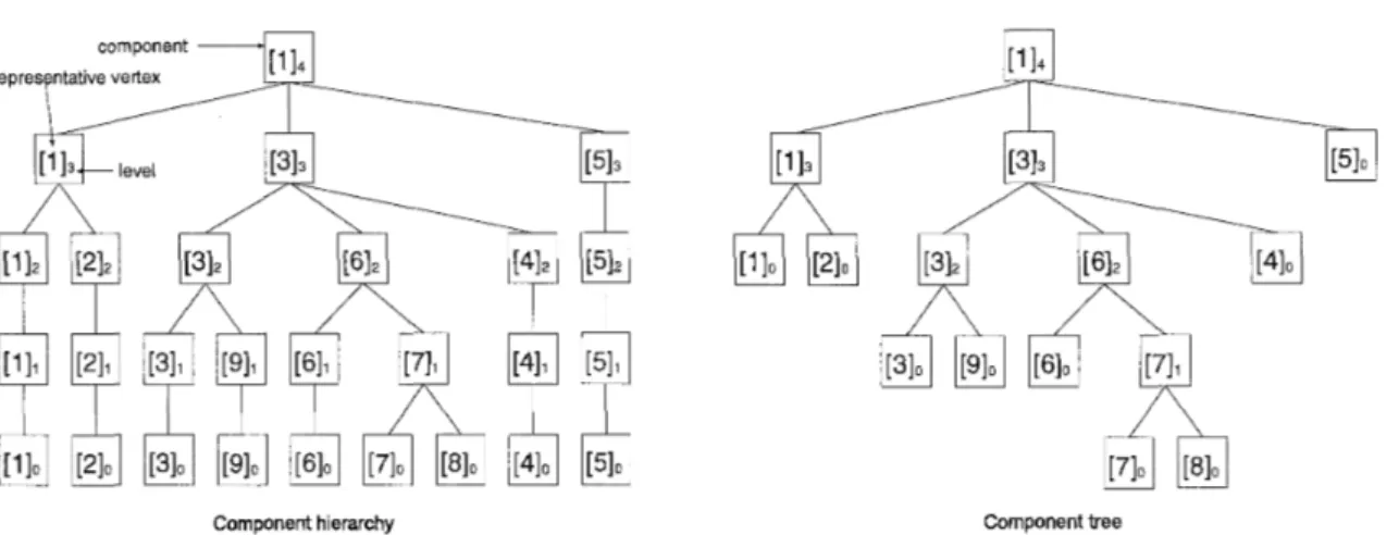
3.1.2. Component tree
T
We denote by Gi the subgraph of G whose edge set is defined to be {e
1
t{e)<
2', e G E}.Thus,
C&
consists of singleton vertices and Gb = G , where b is a word length with f(e)<
2b for all e G E. A maximal connected subgraph of Gi is called a component of Gi. Then the component hierarchy expressing a hierarchy structure of the components is defined as follows:On level i in the component hierarchy, we have the components of Gi. The component on level z containing a vertex v is denoted [vIi. The children of [vIi are the components
{ [ w ] ~ - ~
I
[ w ] ~ = [ v ] ~ (i.e., W G [ u ] ~ )}.
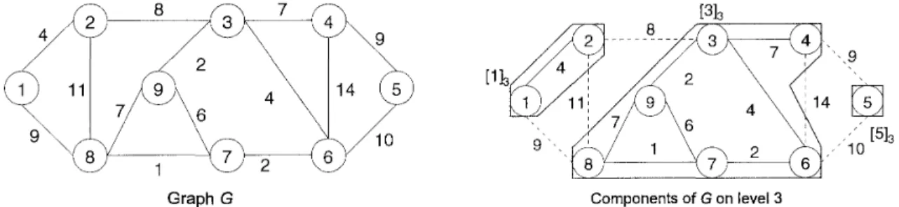
Figure 1 illustrates an example of components of a graph.Graph G Components of G on level 3
Figure 1: A graph G and its components [113, [313, [513 on level 3.
The component tree
T
is obtained from the component hierarchy by skipping all nodes [vIi with [vIi = Thus the leaves of T are the singleton components [vIo = v (v E V) and the internal nodes are the components [ v ] ~ with i>
0 and [ u ] ~ - ~ C The root inT
is the node [ v ] ~ = G with r minimized. The parent of a node [ v ] ~ is its nearest ancestor distinct from [vIi in the component hierarchy. Thus, each internal node in T has a t least two children, and therefore, the total number of components inT
is a t most 2n. We use the component treeT
t o obtain the parent-child relations of the components in the algorithm. Figure 3.1.2 illustrates the component hierarchy and the component treeT.
As observed by Thorup, we can construct the component tree
T
by using only edges of the MST as follows.Efficiency of Linear-time SSSP Algorithm 435
Component hierarchy Component tree
Figure 2: The component hierarchy and the component tree
T
for G in Figure 1. Construct7
Let e ~ j (1
<
j5
n - 1) be the edges of the MSTM ,
and let bMj be the mostsignificant bit of t(eu,) (i.e. bMj = \log,l(eMj)\, and 1
<
bMj<
h). By using packed merging sort [2], make the edge set E, = { e d M I = i7 1<
j<
n - l} for 1<^
i<^
b. Start from the n singleton components (of Go).For i = 1 to b do the following.
(a) Make all components of
G i
from the current component and E, by using union and find [7], t h a t is, if an edge e E E, connects two components (then a new com- ponent of Gi is constructed), make a parent-child relationship in the component treeT .
Problems and our modifications to implement packed merging sort and union and find will be given in Section 3.2.2.
3.1.3. Buckets
B
The buckets
B
consist of multi-level buckets t o maintain the components according to their super distance, and are used as a technique allowing to visit a next node directly without searching onT.
In Thorup's algorithm, we maintain the super distance D(v) for all vertices as Dijkstra's algorithm, and set D ( s ) = 0 and D ( v ) = CO for all v
#
S (v E V) a t first. Note t h a t the value of D ( v ) will change (decrease) in the algorithm when we visit the vertex v as described in Section 3.1.4 (change operation), and when the algorithm terminates D ( v ) will be equal to d(v) for all v E V, similarly to Dijkstra's algorithm. Let D(v) 4, i =\YJ
and D ( X ) = {D(u)1
U C X} for X2
V. Thus, m i n D ( X ) = minuex{D(u)}. D ( v ) 4, i is called a scaled super distance of v. We also use D ( X ) $ k = {D(u) $ k1
U E X} andmin D ( X ) J. k = minuex{D(u) $ k}. We define k-scaled minimum super distance of the component [v], (or [v],) as min £>([v], $ k (or min D([v];) J. k, respectively).
In Thorup's algorithm, we place in the buckets of [v]i, its every child component [ u ] ~ , us- ing a finite value min D ( [ u ] ~ ) $ (?- l) as an index. For example, see Figure 3.1.3 and consider the following case: rnin D([l13) = 0, min D([3I3) = 19, min D([5lO) = 22, min D([lIo) = 0, and min D([2Io) = 4, for the components in
T
in Figure 1. Then min D([lI3) J. (4 - 1) = 0, and rnin D([3I3) 4, (4 - 1) = min D([5Io) $ (4 - 1) = 2, and therefore,[lk
is in the 0-th bucket of [lI4, [313 and [5Io are in a 2-nd bucket of [lI4. Similarly, min D([lIo) J. (3 - 1) = 0,(and rnin D([2Io) J- (3 - 1) = l ) , and therefore, [ll0 is in the 0-th (and [2lO is in the 1-st) bucket of [113, respectively.
Y. Asano & H. Imai
index buckets
Figure 3: Illustration of the buckets B. Parts below [3]3 is omitted for simplicity. Note that in the algorithm we place only components which have finite min D in the buckets of its parent, and therefore, a t first of the algorithm, only the root component of
T
and components which contains the source s are inB
since D ( s ) = 0 and D ( v ) = oo for v # S (ve
V).To construct
B,
we have only to compute the width of the buckets for each component before we place the components. The width of the buckets of [vIi is bounded by (max d([vIi) -min d ( [ v I i ) ) / 2 " l
,
and (max d([vIi) - min d([v]i)) is bounded by the diameter of [ u ] ~ (thediameter of a connected graph is the length of its longest path). We can observe that the total number of the buckets is bounded by 8n, as observed by Thorup [10]. The fact is important for the space complexity of the algorithm.
3.1.4. Interval tree U
U is called (the set of) unvisited children in [10], but in this paper we call it an interval tree, since a structure of U is an interval tree from the implementation point of view. T h e interval tree U maintains values D(v) of the vertices and min D of unvisited components which contain visited parents t o place the components correctly in B. This is the reason t h a t Thorup named U unvisited children.
First, we explain the structure of U. The interval tree U is a d a t a structure for only computing min D of the unvisited components efficiently, and therefore the structure of U is quite far from the conceptual image of U (in Figure 5). In U, we use another ordering of the vertices {ul, . . .
,
un}, which is a permutation of {l, . . .,
n} satisfying the following condition: (i) the root component ofT
consists of {ul,
.. .,
un}, (ii) if a component consists of a sequence{ui, u;+l, ..., uj-1, U)} and it has k children Xi, ..., X k (i.e. X i is the leftmost child and X k is the rightmost child in
T ) ,
and lXhl = xh (1<
f t $ k ,xLl
xh = j - k+
l ) , then X hconsists of a sequence {urn ...
,
ub} where a = x h+
i , b = a+
xh - 1. For example, forT
in Figure 2, the root [lI4 consists of {ul, ...,
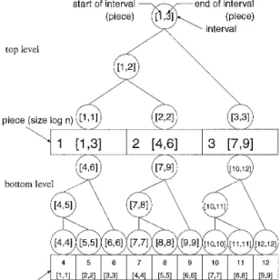
u9}, and its children [lI3, [3]3, [510 consist of {ul,u2}, {us, ..., ua}, {us} respectively, since l[ll31 = 2, l[3l31 = 6, l[5lo1 = 1. We call segment[a, b] corresponds t o a component X if X consists of a sequence {ua, ..., ub}.Figure 4 shows the structure of U for n = 9 (it depends on only the number n ) . For example, a p i e c e d ) (a rectangle with 1 and [l, 31) is a super vertex for vertices u l t o us
,
and a piece(2) ( a rectangle with 2 and [4,6]) corresponds t o vertices u4 t o U @ , and a piece(4) (a rectangle with 4 and [l, l]) corresponds to vertex ul respectively. At the top level, a piece corresponds t o [log2 n] vertices, and at the bottom a piece corresponds t o [log2 log2 nJ vertices. Furthermore, a circle with [l, 31 means an interval contains pieces pieced) t o ~ i e c e ( 3 ) , and thus it contains a sequence { U \ , . . .,
ug }. We call the circle interval([l, g]),Efficiency of Linear-time SSSP Algorithm
and call a circle with [2,2] ([7,8]) contains a pieced) (piece(7) and piece(8)) interuals[4,6] (interual([7,8])), respectively. Note that in this figure since n is small, a piece in the bottom of the figure corresponds a vertex.
Now we discuss the size of the interval tree, U. At the top level of U we deal with 1log n) vertices as one piece, so that the number of the pieces of the top level is a t most n / [\og n \ .
Then a t the bottom level, we construct an interval tree for each piece of the top level, and in this tree we deal with 1log log n\ vertices as one piece, so that the pieces of the bottom level are a t most
n/
[loglogn]. Thus, the total number of nodes (drawn as circles in Figure 4) in U is bounded by 2n since a t the top level there are a t most 2n/ l o g n nodes and a t the bottom level there are a t most 2n/ 1log log n] nodes. Thorup used a Q-heap [6] t o implement each bottom piece (which contains a t most log log n vertices), and we can construct U in 0 ( n ) time if we could implement the Q-heap on today's computers, but the Q-heap is too complicated to implement, and therefore we discuss this problem in Section 3.2.3.start of interval end of interval (piece) interval
top level
bottom
piece (size log log n)
Figure 4: The interval tree U for n = 9.
The interval tree supports two operations called change and split t o maintain min D([uIi) of every components dynamically in the algorithm.
First, the change operation corresponds t o the updates of D when a vertex is visited in Step 2(b) of Dijkstra's algorithm (thus, the total calls of change is a t most m ) . When we visit a vertex U , for each vertex W adjacent to U we perform the change(w) operation to update min D([wIi) where [ w ] ~ is a component in U, and t o relocate the component [ W ] , in
the buckets of its parent.
Next, we describe the split operation, more difficult and complicated one. When we visit a component, components t o be maintained by U (i.e., unvisited components having a visited parent) may change' and we must recompute min D of new elements of U to place the unvisited components in proper buckets in
B.
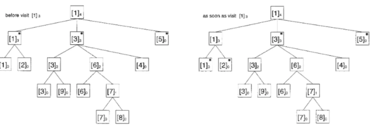
Figure 5 shows a conceptual image of the split operation. Components with asterisks in the left figure are maintained by U before we visit [lI3. As soon as we visit [l]3, the domain is changing to components with asterisks in the right figure. Then, we compute min D([lIo) and min D([2Io).438 Y. Asano & H. Imai
before visit [l] 3
1
as soon as visit [ l 1 3Figure 5: Illustration of the changes of the domain (i.e., split).
We explain an implementation of the split operation using the data structure of the inter- val tree. For the split operation we have to compute rnin D of new elements maintained by
U, by using interval tree. Since when we require to compute rnin D([U];) for some component u ] ~ , instead of searching D(w) for all vertices W E [v]$, we compute rnin D of some intervals. An interval[a, b] is said to be unbroken when it is contained in some segment[c, d] (i.e. a
>
c and b <_ d ) corresponding to some component maintained by U. We can compute rnin Dof components maintained by U, by comparing all maximal unbroken intervals contained in segments corresponding to the components, and we can find the maximal unbroken in- tervals by searching down from the root. Let min D(interval[a, b]) denote m i n a < i < b { D ( ~ j ) } and rnin D(piece(a)) denote min,, emccew { D (U,}
1.
We can compute rnin ~ ( $ e r v a l [a, b]), by computing rninc<hSd D(piece(h)) if piece(c) to piece(d) are contained in the interval. Note that rnin ~ ( p i % e ( a ) ) for piece(a) in the bottom level can be obtained by a Q-heap in constant time though it has l o g log n\ vertices.For example, for
7
in Figure 2, a t first only [lI4 is maintained by and a maximal unbroken interval is interval[l, 91, the root of the interval tree, and when we visit [l]4, to place its children in the buckets, we split [lI4. Then, [ 1 ] 3 , [3]3, [510 (i.e. segment[l, 21, segment[3,8], segment[9, 91 respectively) are maintained by U now, and by searching down the interval tree, maximal unbroken intervals are interval[l, 21, interval[3,3], interual[4,6], interval[7,8], interval[9,9]. We compute rnin D[lI3 from rnin D of interval[l, 21, and min -D[3l3 from interval[3,3], interval [4,6], interval[7,8], and so on. Furthermore, when we split113, then [lIo, [2Io, [313, [5Io are maintained by U, and therefore maximal broken in- tervals become to interval[l, l], interval[2,2], interval [3,3], znterval[4,6], znterual[7,8], interval[9,9]. Then we only compute rnin D of interval[l, l] and interval [2,2], and do not need to recompute the others.
3.1.5. Visit
For (e), this part is the search phase and a main routine in the algorithm. Let us call the part visiting-part from now on, since we visit components in the component tree. We can solve SSSP with the source s by calling Visit ([sir, r
+
1) recursively described below where r denotes the level of the root ofT .
Visit ([v];, j ) : We assume the parent of [ v ] ~ is [v], ( j
>
2).1. If i = 0, then for each vertex W adjacent to v, update D ( w ) just like Dijkstra's algorithm, and perform the change(w) operation of U. Then, exit the call.
2. If we have not called Visit ([v];, j ) previously, do the following (a)-(c) .
Efficiency of Linear-time SSSP Algorithm 439
(b) Place the children [ u ] ~ t o the bucket of ([U],) along min D([uIh) J, (i - 1). (c) Set index := min £)([U], J, (i - 1)
3. Repeat the following (a) and (b) until we have visited all vertices in [ u ] ~ or index J,
( j - i) is increased:
(a) While there are children [wIh in a bucket with min D([w]i,) = index, do the following.
i. Let [wIh be such a child component in the bucket. ii. V i s i t ( [ w h , i) (recursive visiting).
(b) Increase index by one.
4. If we have visited all vertices in [ u ] ~ , delete [U], from the bucket of the parent.
5. Otherwise, replace [U], in a proper position of the bucket of the parent using new min D ( [ U ] % ) .
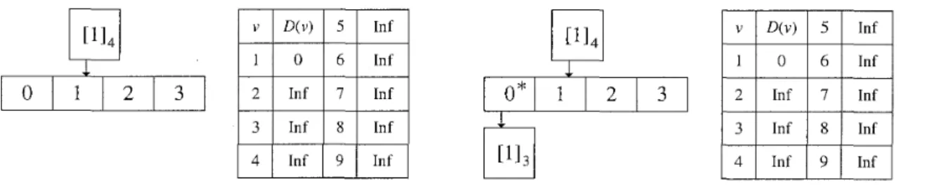
Figure 6 t o 8 illustrate a beginning part of the algorithm V i s i t for
G
in Figure 1 and'T
in Figure 2. At first, when Visit([lI4, 5) is called, the buckets of [lI4 are empty, and D ( 1 ) = 0, D(v) = cc for 2<
U<
9 in the left part of Figure 6. Then, we perform split t o place children of [lI4 in the buckets, and therefore, U maintains [113, [313, [5Io now. Since only [1J3 has a finite value min D([lI3) J, (4 - 1) = 0, [l13 is placed in the 0-th bucket of [lI4,and an index for the buckets of [lI4 is set to 0. See the right part of Figure 6, the asterisk signifies the index.
Then V i s i t ([113, 4) is called, and by splitU maintains [1l0, [2Io, [313, [5Io now, and [lIo is placed in the 0-th bucket of [lI3, and an index for the buckets of [lI3 is set to 0, as the left part of Figure 7. Then V i ~ i t ( [ l ] ~ , 3) is called, and by the changed) operation and scanning edges adjacent to the vertex 1, D(2) = 4 and D(8) = 9 now. Since [210 and [313 in U have finite values min D([2Io)
4.
(3 - 1) = 1, min D([3I3)-1.
(4 - 1) = 1, respectively. Then since[lIo becomes empty, it is deleted from
B,
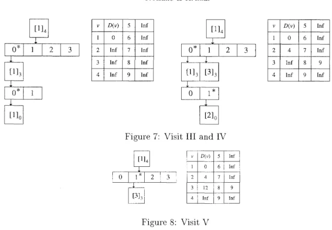
and the index for the buckets [1J3 increases by one, as the right part of Figure 7.Then V i s i t ([llo, 3) is called, and by the chanqe(2) operation and scanning edges adjacent to the vertex 2, D ( 3 ) = 12 now, but a value min D changes for no component in U. Then since [2Io becomes empty, it is deleted from
B,
and the index for the buckets Ill4 increases by one, as Figure 8. We omit the reminder of the algorithm.1
;
1
1
;
1
In f Inf1
Figure 6: Visit I and I1The time complexity of the algorithm is O ( n + m ) since each call for V i s i t must determine d(v) for some U <E V or increase the index of the buckets by a t least one, where the total number of buckets in B is a t most 872, and the split and the change operation are called a t most n and m times, which can be performed in 0 ( n ) and 0 ( m ) time respectively, as proved by Thorup.
3.2. Our m o d i f i c a t i o n s
We describe the problems arising in implementing it to run on today's computer, and then, we propose modifications. The main reason of difficulty in implementing Thorup's algorithm
Y. Asano & H. I m a i
Figure 7: Visit I11 and IV
Figure 8: Visit V
is data structures used in the linear-time MST algorithm. The data structures atomic-heap and Q-heap, which are proposed in [6], need a huge word-length.
3.2.1. Modifications of atomic- heap and Q-heap
T h e atomic-heap is a list of heaps like the Fibonacci heap
([5]).
An array called forest buckets maintains the root of heaps like the root-list of the Fibonacci heap. More precisely, the forest buckets consist of 12 buckets each with size (log n)'I5, and therefore, the number of elements in the forestbuckets can be ^(log n)'I5. The problem is that in [6] a Q-heap, which can have a t most (logn)lI4 items as described below, maintains the forest buckets, thus we need n>
21220 to satisfy (logn)'I4>
1 2 ( 1 0 ~ n ) ~ / ~ . Thus we propose that we use a Q-heap for each bucket (i.e., 12 Q-heaps for the forest buckets). After t h a t we require a cost larger by a constant factor 12 to find the minimum element from the atomic-heap, but we are free from the limitation of n .Q-heap is a d a t a structure like priority-queue, and to perform all of heap operations in constant time, although its size is limited by only [(log n)'I4J, and moreover, it uses too complicated a table-lookup method to implement. Thus, we propose that we use an array of size 2 instead of the Q-heap since the size 1(logn)'l4] 5 Lb'14J
5
2 where b denotes the word length and b = 32 or 64 on today's computers. This modification does not break the constant-time complexity on today's computers.3.2.2. Modifications in construction of T
We have some small problems to implement the construction of
7'.
First, in the construction of T , Thorup used a packed merging sort proposed in [2] and [l]. It is too complicated t o implement, but in this problem it is used only for n<
b and for other n the bucket sort is used. Therefore, we assume n>
b t o avoid the packed merging sort. This causes almost no problem for most applications. Next, Thorup used a linear-time u n i o n and find algorithm proposed in [7] t o construct7
fromM
of (n - 1) edges and n vertices. It is toocomplicated to implement and we decide to use the union with size and the find with path compression instead of the algorithm, since the time complexity of the path compression
Efficiency of Linear-time SSSP Algorithm 441
method is 0 ( a ( n , n ) n ) , where
a(n^
n ) is the functional inverse of the Ackerman function 265536a n d a ( n 1 n ) < 4 f o r a l l n < 2 .
3.2.3. Modification of U
The remaining problem t o implement the algorithm is the interval tree U. The interval tree U is realized as a two-levels tree in [10]. The problem is t h a t we must maintain the bottom super vertex with a Q-heap in [l01 t o perform all operations of heap in constant time. Recall that a Q-heap can maintain only a t most (log n)'I4 elements (in our methods, the upper bound of the size is equal to 2 as above), and that it needs (log n)'I4
>
log log n. Since this inequality is satisfied only when n>
2216, we cannot implement the interval tree with a naive method on today's computers.To cope with this problem, we propose t h a t we implement the interval tree as a three- levels tree. Under the second level of the tree, we attach a third level similarly in which each super vertex is for Ilog log log n vertices. The Q-heaps maintain the super vertices in the third level only. Then, since 1log log log n
5
2 for n<
264, we can maintain the super vertex by a Q-heap with size 2 on today's computers.3.3. Summary of experimental results for t h e whole algorithms
By using these modifications we are ready t o implement Thorup's linear-time algorithm.
In fact, we have actually implemented the algorithm together with the supported d a t a structures and measured execution times of the implementation. We also implemented old algorithms based on Dijkstra's algorithm to compare the practical efficiencies. We note t h a t the program (written with C++) is over 3,000 lines (c.f. naive Dijkstra program is only 100 lines), and this complexity of the program does not make merits in practice with comparing other implementations.
Here we only summarize results of the above experiments. For the whole execution time for SSSP (instead of search time), Thorup's algorithm take more time than the algorithm based on the Fibonacci heap in [5] (i.e., Dijkstra's algorithm with the Fibonacci heap which has time complexity O ( m
+
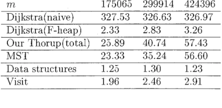
n log n ) and is the theoretically fastest algorithm based on the comparison computation model today). In particular, the part of the MST algorithm occupies most of the execution time of Thorup's algorithm. Table 1 shows the running times of Thorup's algorithm and Dijkstra's algorithm (naive one and one with Fibonacci heap) on random graphs n = 50000, m = 175065,299914,424396, respectively, and rows MST, Data structures, Visit show times to construct the MSTM ,
the other d a t a structures(7,
B,
U), and times for Visit ( [ s ] ~ , r+
l ) , respectively. For experiments, we use Sun Ultra 30 workstation with 1GB main memory. Our programs are written in C++.Table 1: The running times (sec) of Thorup's algorithm and Dijkstra's algorithm (naive and Fibonacci heap versions), n = 50000
m 175065 299914 424396 Dijkstrafnaive) 327.53 326.63 326.97 Dij kstra(F-heap) 2.33 2.83 3.26 Our Thorup(tota1) 25.89 40.74 57.43 MST 23.33 35.24 56.60 D a t a structures 1.25 1.30 1.23 Visit 1.96 2.46 2.91
442 Y. Asano & H. Imai
For space, we require a t most 56n words for
7"
and a t most 32n for the buckets and a t most 34n words for U in our implementation. Thus, our implementation requires a t most 122n words (except the space for the graph and the MST). Note that we do not discuss memories for the MST, since the MST can be free after the construction of the MST.The results above concern with the single query mode problem. Thus, it is too early t o say that Thorup's algorithm is not useful in practical applications since it can be used as the shortest path search problem. In the next section, we analyze the visiting-part (search phase) and clarify the possibility of the usefulness of Thorup's algorithm a
4. Analysis of the Visiting-part
The visiting-part is important for practical use since only the visiting-part is repeated for each query source in the shortest path search problem. If the execution time of the visiting- part is less than the whole execution times of other algorithms based on Dijkstra's one, our implementation based on Thorup's algorithm will be useful for the shortest path search problem. In this section we show the details of the visiting-part and analyze it theoretically and experimentally.
We can divide the visiting-part into the 3-parts as follows. Refer section 3 for the algorithm of the visiting-part.
1. Main routine of visiting (Visiting-main or VM for short)
Scanning the buckets of the component from left t o right, we visit the children compo- nents in the buckets (we call the procedure Visiting-main-body or VMBD for short). Then, if necessary, we replace the component in the appropriate bucket of its parent as described in page 9, step 5 of Visit algorithm (we call the procedure Visiting-main- bucketing or VMBC for short). Quantities concerning the procedure VM are the total number of the buckets (at most 8n) and the number of the components (at most 2n). Note t h a t the number of calls of the procedure depends on the order of visiting (and also depends on the source).
2. Visiting the leaves (Visiting-leaves or VL for short)
When visiting a vertex (leaf of
T),
we scan the vertices adjacent t o the vertex and changes D of the vertices properly as in Dijkstra's algorithm (Visiting-leaves-Dijkstra or VLD for short). The total calls of the procedure is always n , and the total number of the changing D is bounded by m. Concerning the changing D , we perform the operations change of U (Visiting-leaves-change or VLC for short), and then, if neces- sary, we replace components which have updated min D in buckets of their parents (Visiting-leaves-bucket or VLB for short).3. First bucketing for each component (Expand or EX for short)
When we visit a component for the first time, we place its children components t o its buckets (Expand-bucket or EXB for short). At this time, we perform the operation split of U (Expand-split or EXS for short).
The total calls of the procedure and split is equal t o a difference between the number of the components and the number of the leaves in
T,
that is, (the number of the components - n). Note that the number of the elements of U (intervals, pieces, muiin Figure 15) concerns the total execution time of the procedure. For details of the elements of U, see [10].
Note that the execution time of the whole of the visiting-part (VW for short) is equal to the sum of the execution times of VM, VL, and EX.
Efficiency o f Linear-time SSSP Algorithm 443
We measure the execution times and the number of calls of the three parts and the sub procedures and the numbers of the elements by several experiments. In addition, we compare the execution times of the visiting-part with the execution times of Dijkstra's algorithm with the Fibonacci heap (F-heap, for short) and the algorithm with the binary heap (B-heap, for short). We note that Dijkstra's algorithm with the binary heap proposed in [l11 is very popular in practice and it has O ( m log n ) time complexity for the worst case. Refer [3], [8], and [g] to acquire the efficiency of the binary heap comparing with other algorithms and data structures.
We use five random graphs and five k X k grid graphs in the experiments. We make the
random graphs for given n (V = {l, ..
.,
n}) and m as follows (in the following experiments, we fix m = 5n).1. We assume that there are edges (i, i
+
1) for all i = 1, . . .,
n - 1. The assumption is forconnectivity, and it does not lose the generality.
2. For the remaining m - n
+
1 edges, there are n(n - 1)/2 - ( n - 1) = ( n - l ) ( n - 2)/2combinations
(4
j ) . Let L E denotes a number of remaining edges and LV denotes a number of remaining combinations.3. For (1,3) to (n - 2, n ) , we give a possibility L E / L V for an edge.
We use uniform random numbers from 1 to 100 for the weights of the edges of the random graphs and the grid graphs. We note that the graphs are sparse (m = 0 ( n ) ) since if m = 0 ( n 2 ) the time complexities of any algorithms are equal and if m = O ( n log n ) Thorup's algorithm and Dijkstra's algorithm with the Fibonacci heap have the same time complexity. The results obtained by the experiments are given below with the boxplots. In the figures, the left graphs correspond to the grid graphs and the right graphs correspond to the random graphs.
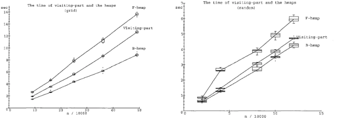
7- s e c 6- - 5.- 4.- 3-- 1- 1.-
The time o f visiting-part and the heaps (random)
Figure 9: The execution times of the visiting-part, the Fibonacci heap algorithm (F-heap) and the binary heap algorithm (B-heap).
From the experiments, we obtain the following observations.
Visiting-part is as fast as the heaps (faster than F-heap and slower than B-heap). Note that the time complexity B-heap is now O ( n log n) since we use m = O(n). The times of them are roughly proportional to n in the experiments. More precisely, in the grid graphs, the execution time of the visiting-part is less than 0.30 X 1 0 4 n (note that m = 2n) and the time of B-heap is more than 0.0090 X 1 0 4 n l o g n , and thus,
the visiting-part is faster than B-heap only when logn
>
0.30/0.0090, that is, roughly n>
234. In the random graphs, m = 672, the execution time of the visiting-part is lessY. Asano & H. Imai
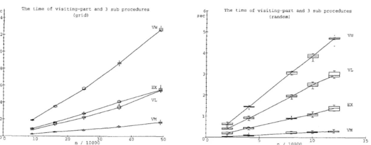
The time of visiting-part and 3 sub procedures The time of visiting-part and 3 sub procedures
(grid) (random)
5 l
1 i n n n n 10 15
Figure 10: T h e execution times of the visiting-part (VW) and its 3 parts procedures VM, VL, EX.
The time of visiting-main and its sub procedures (grid1
1 The time of visiting-main and its sub procedures s e d (random) VM VMBD VMO VMBC 15
Figure 11: The execution times of Visiting-main (VM) and its sub procedures (VMBD, VMBC described as above, and VMO denotes the other remaining procedures in VM except VMBD and VMBC, t h a t is, Visiting-main-others).
than 0.45 X 1 0 4 n and the time of B-heap is more than 0.018 X 10^^nlogn, and thus,
the visiting-part is faster than B-heap only when logn
>
0.45/0.018, that is, n>
225. Note t h a t in dense graphs B-heap has less advantages than in sparse graphs. As a result, on today's computers, the visiting-part is not faster than B-heap. Note t h a t our implementation of Thorup's algorithm needs more than lOOn words of memories as described in previous section.VL (Visiting-leaves) and EX (Expand) occupy most of the time in the visiting-part, though VM (Visiting-main) takes small time (figure 10).
VLD (Visiting-leaves-Dijkstra) and VLC (Visiting-leaves-change) occupy most of the time in VL, and VLD takes more costs than VLC (figure 12).
EXS (Expand-split) occupies most of the time in EX (figure 13).
As a result, VLD, VLC, and EXS occupy most of the time in the visiting-part. Note that VLC and EXS are the operations of the interval tree U, and VLD is the same operation as update D in Dijkstra's algorithm, which implies we can hardly reduce the times of VLD.
The total numbers of calls of all the procedures are proportional to n (figure 14) since we fix m = 0 ( n ) for the experiments. This result confirms the theory. Note that calls
Efficiency of Linear-time SSSP Algorithm
fi- The time of visiting-leaves and its sub procedures (grid)
The time of visiting-leaves and its sub procedures (random) VL VLD VLC VLB 2LQ.-
Figure 12: T h e execution times of Visiting-leaves (VL) and its sub procedures VLD, VLC, VLB, and Visiting-leaves-others (VLO) similar to VMO.
The time of expand and its sub proceduresEx The time of expand and its sub procedures
(grid) (random)
Figure 13: The execution times of Expand (EX) and its sub procedures EXS, EXB, and Expand-ot hers (EXO) .
of VM is more than calls of VLC in the grid graphs, on the other hand, in the random graphs calls of VM is far less than calls of VLC, since calls of changes increases when m is larger.
The number of all the elements are proportional t o n (figure 15). This result confirms the theory.
Finally, we discuss the results and future works in next section. 5. Concluding Remarks
In conclusion, our implementation of Thorup's linear-time algorithm is very slow for SSSP
due to the time of the construction of the d a t a structures. On the other hand, the uisiting- part, which is repeated in the shortest path search problem, is as fast as the algorithms using the heaps.
Thus, due to the huge amount of memories and the complicated and large programs, our implementation of Thorup's linear-time algorithm is not useful in practice today.
However, we should make clear which parts in the visiting-part are slow for more improve- ments in the future. We note that the bottlenecks in the visiting-part are Visiting-leaves and Expand parts, and therefore, if we can improve the parts, we can acquire a faster im- plementation. In particular, we can modify the implementation of the interval tree U t o
446 Y. Asano & H. Imai
The total numbers o f the calls h t o t a l numbers of the calls
l random1
VLB
/ VLC
Figure 14: The total numbers of the calls. Note that the number of VM is equal to the ones of VMBD and VMO, similarly, VL is equal t o VLD and VLO, EX is equal to EXS and EXO- Further. VL is eaual to n.
The numbers of the elements (grid)
+- # of buckets
-A-# of components
Th~numbers of the elements (random)
600000
1
-+ + # of edges (m) # of buckets + # of components -x- # of intervals 400000 -a- # of pieces 0) L2S
200000 - 0Figure 15: The numbers of the elements. Note that intervals, pieces (correspond to the super vertices), and mui (maximal unbroken intervals which belong to the components to find the minimum D by scanning, refer [l01 for a detail) are the elements of the interval tree
U.
improve Expand part (i.e., split), for example, changing the structure. In this paper, we use the three-levels interval trees and its super vertices have sizes log n , log log n , and 2, but we can implement it with other methods changing the number of levels and the sizes of the super vertices. Moreover, we will be able t o reduce the amount of memories by using some minute techniques, in particular, in
'T
and U.Finally, we describe the future works.
o Can we improve the implementation of Thorup's algorithm for practical use?
Can we use the idea that we divide the algorithm into the preprocess constructions of the d a t a structures and the visiting-part, to make a more efficient algorithm?
o Can we apply the d a t a structures in [l01 to other problems?
References
[l] S. Albers and T. Hagerup: Improved parallel integer sorting without concurrent writing. Proceedings of 3rd ACM-SIAM Symposium on Discrete Algorithms, (1992) 463-472. 2 A. Andersson, T. Hagerup, S. Nilsson and R. Raman: Sorting in linear time? Proceed-
Efficiency of Linear-time SSSP Algorithm
ings of 27th ACM Symposium on Theory of Computing, (1995) 427-436.
[3] B. V. Cherkassky, A. V. Goldberg and C. Silverstein: Buckets, heaps, lists, and mono- tone priority queues. Proceedings of 8th ACM-SIAM Symposium on Discrete Algo- rithms, (1997) 83-92.
[4] E. W. Dijkstra: A note on two problems in connection with graphs. Numerische Mathematik, 1 (1959) 269-271.
[5] M. L. Fredman and R. E . Tarjan: Fibonacci heaps and their uses in improved network optimization algorithms. Journal of the A CM, 34 (1987) 596-615.
[6] M. L. Fredman and D. E. Willard: Trans-dichotomous algorithms for minimum span- ning trees and shortest paths. Journal of Computer and System Sciences, 48 (1994) 533-551.
[7] H. N. Gabow and R. E. Tarjan: A linear-time algorithm for a special case of disjoint set union. ~ o u r n a l of Computer and System Sciences, 30 (1985) 209-221.
[8] A. V. Goldberg and C. Silverstein: Implementations of Dijkstra's algorithm based on multi-level buckets. Technical Report 95- 187 (NEC Research Institute, Prinston, N J ,
1995).
[g] H. Imai and M. Iri: Practical effeciencies of existing shortest-path algorithms and a new bucket algorithm. Journal of the Operation Research Society in J a p q 43 (1984) 43-58.
[l01 M. Thorup: Undirected single source shortest paths in linear time. Proceedings of the 38th Symposium on Foundations of Computer Science, (1997) 12-21.
[l11 J. Williams: Heapsort. Communications of the ACM, 7 (1964) 347-348. Yasuhito Asano
Graduate School of Information Science The University of Tokyo
7-3-1, Hongo, Bunkyo-ku, Tokyo 113-0033, Japan
![Figure 3: Illustration of the buckets B. Parts below [3]3 is omitted for simplicity](https://thumb-ap.123doks.com/thumbv2/123deta/5788168.1527905/6.892.292.532.123.357/figure-illustration-buckets-b-parts-omitted-simplicity.webp)