On the Equilibrium Probabilities of GI/G/l

(1)

]. Operations Research Soc. of japan Vo!. 10, Nos. 3 & 4, June 1968

ON THE EQUILIBRIUM PROBABILITIES OF GI/G/l

YOSHIRO TUMURA Science University of Tokyo

(Received November 30, 1967)

1. Introduction

In the previous paper we have developped the equilibrium equations method on the most general queueing system [3]. As applications of the theory we could obtain the equilibrium probabilities and others in the simple cases as M/C/I(oo), CI/M/m(oo), CI/M/m(N), Cl/Et/I, etc. In the present note we shall give the solutions of CI/ M/m and

CI/C/l(oo) system. Consider the many servers system. Let A(r) be the distribution function of the inter-arrival time and B(s) that of. the service time, both satisfying the following conditions: (1I) A(r) and B(s)

are absolutely continuous except at most the sequences {'v} and {sv} respectively, where {rv}and {sv} have not any finite cluster point. Fur-thermore, means

exist.

In [3] we assumed the conditions (I) and (Ill) in addition to (11), but in the simple cases as CI/C/l and CI/ M/m (I) is necessary attained and (Ill) is simplified by J..<p. in the case CI/C/I( (0) or J..<mp. in the case CI/M/m(oo).

Let {tn } be the sequence of instants when customers arrive, and in

the case CI/C/I {tn'} that when services begin, and in the case CI/C/I

Po(r; t)= P,. {1/(I)=O, ,:::::;r(t)<~+tI,}

/a"

93

(2)

94 Y. 7'umura

Pn(r,S; t)=Pr{"'J(t)=n, r;:;;-r(t)<r+or,s;:;;s(t)<s+os} /oros,

(n~l)

in the case GI/M/m

where and Pn(r; t)=Pr{"'J(t)=n,,, :;;;z(t)<r+or} /or, (n~O) r(t)= min (t-tn)

'n:a'

s(t)= min(t-tn'), 'n':;;t

and 1)(t) is a random variable denoting a number of customers in the system at the instant t. In these simple cases we have already obtained

Theorem. If the system satisfies the condition (11) and the inequality ).<1' (in the case GI/G/l(oo» or l.<mf (in the ca$e GI/M/mCoo», then'

( i ) in. the aperiodic case, the limit

~

GI/G/l

!

GI/ M/m

"""""""""""""""""""""""""""",,,,,,,,,,,,,,,,,,,,,,,,,,,,,,,,,,,,,,,,,,,,,,,,,,,,,,,,",

and

~

Po(r; t)=Po(r)

I

lim Pn(r; t)=Pn(r)

: lim Pir,s; t)=Pn(r,s) !.

t ... oo ~

exist and satisfy the equation

00

(1)

E

Pn=l,

0=0

where

(3)

0" the Equilibrium Probabilities of GI/G/l IJS

In the periodic case with period w, Po(r;t), Pn(r,s;t), Po(r),Pn(r,s) [or Pn(r; t), Pn(T)] and Pn are to be replace merely by Po(T; t), Pn(r,s; t), Po(r), Pn(r, s) [or Pn(T; t), Pn(r)] and Pn , where

PO(T; t)=-1

)'+"

Po(r; t)dt, w 1

Pn(-r,s; t)=-

11'

+" Pn(T,S; t)dt.

w 1

(ii) poeT) and Pn(T,S) [or Pn(T)] satisfy the equilibrium equations shown in 3 [or in 2].

(iii) the equilibrium equations have an unique non-trivial solution; that is, non negative and satisfying (1).

(iv) the equilibrium probabilities q~ at the arrival time {tn} are given by

1

r

dA(T)

qo=

TJ

poeT) I-ACT)' qk=

TJ

1

r

P,,(T) I-ACT)' dA(T) and

1

r

dA(T)

qk= TJPt{T,S) l-A(r)ds.

in the aperiodic case. In the periodic case Plc must be 'eplaced by Plc.

On the other hand, if the equilibrium equations satisfying the con-dition (ll) have non trivial solution, thtm the system satisfies also l<p

[or l<mp].

Hence, it is sufficient to find a set of solution satisfying the equations.

2. GIIMlm

2.1. At first consider CII Mlm( 00) system which has been solved by L. Takacs [2]. The equilibrium equations in the aperiodic case are in the following:

(4)

96 Y. Tumura

for r~O,r.

(1 ) [ : . +A (r)+n,u

]P,,(r)=(~+

1),uPn+1(r) (n=O, 1, "', m-I),

(2) [fr-+A(r)+m,u ]P,,(r)=m,uPIl+1(r)

(n~m),

with initial conditions

(3)

and with (4) where

l-A(r.+O)

PIo(r-+O)=I-=-A(~:-"':::Oyp,,(r.-O) (for all n and v),

A(r)=A'(r)/[I-A(r)] .

The equations (2) with (3) (n~m) have a solution (5) Pn(r)=kan-m[I-A(r)] exp [-m,u(l-a)r] (n~m),

where a is a root of a characteristic equation (O<a<l)

(6) a=A*[m,uCl-a)] ,

A* denoting the Laplace-Stiltje's tronsform of A(r) A*(z) =

~~ e-~<dA(r).

The eqations (2. 1) have a solution*

(7) Pn(r)=k[l-

A(,)(m~~:\

-1)'

(n~v)Cn+.e-(n+»pr

+( _1)m-n m-n m-v+l IT e-mp(l-a)r ]

.,=1

v-ma

(n=O, 1"", m-I),

where constants

Cr,

are determined from (3) (n<m) by the equations

*

It is assumed in (7) and (8) that v-ma (v=I,2, "',m-I) are not zero. If one of v-ma is zero, (7) and (8) would be partially revised.

(5)

On the Equilibrium Probabilitie. of GI/G/l (8)

C",_nA;'_ ..

=

:~:

(-1),-1

Cm_,,+{ (m::;v)+(m-:+IJ)A:'_ .. +v

J

11-1

m-v+l

n-(n 1\~ +(-1),,-1

n ____

-

JU v=1 1'-n:/a n-n:/a' (n=1,2, "',m), where A .. *=A*(np) •

Adding (7) and (5) respectively, we have

and

Hence from

we have

(9)

2.2. Now' P,,(r:) are given, the following results are easy to obtain

mp[",_1

(i)

Po=1-"

I:

(-1)"

(l-Av) +*

Co

"=,

l'

"'n"

_1?! ..

=.:-::±J.]

m v~l 1'-n:/a

(n=I,·· ·,m-I).

(6)

98 or Y. Turnura

m-I

(1 1)

Po=1- p- mp

L:

q.-l - - - - 0 - - - , "=1 V

m

p,.=mPqn_1 (n=1,2,···,m-1),

n

Pn=pq,.. (n~m).

(iii) the probability not to wait is equal to a C_o(1-a)' (iv)

m-I(

_L:

1 - -

v)P

.=1-p.

"=0

m

(v) Let L be number of customers in the system and Lq that in the queue. E{L} pa C_o(1-a)2 ' pa C_o(1-a)2,-\mp, pa(1 +a) p2_a2 Co(1-a)8 Co2(1-a)' .

Let

L/

be a number of customers in the queue at arrival time.

E{Ll} = C_o(1-a)2 '

VeL 1)= a2(1+a) q C_o(1-a)8

(vi) Let Wq be the waiting time of customers. The distribution functions of Wq is given by

ti

F(w)-1 _'--::':' __ e-mp(l-a)w q • q - - C_o(1-a)

(7)

011 the Equilibrium Probabilitie8 of CI/C/l 99

E{W,} _ a

q - mpCo(l-a)l ,

Let W be the time which customers spend in the system. Its dis-bution function is given by

F(w)=

1 ~

[1

+

a Je-·pw

+

a e-mp(l-a)w

Co(1-aXm-1-ma) Co(1-aXm-1-ma)

Remark. (a) in the case M/ M, a= p

( b) in the case GI/ M/1( 00),

Co= l/(l·-a) ,

hence,

Po=l-p

pn=

pa

n-

l_{(l-a) (n;;;;;l),}

and

In the case GI/M/2(00),

1-a-A*

Co= (1-aXl-2a)A* (A*=A*(p)),

hence, p(2-2a-3A*+2aA*) Po=l- 1-a-A* 2,c(1-aXl--2A *)

Pl

= 1-a-A*

P"

pa n - Z(l-a)(l- 2a)A * 1-a-A* (n~2) . (1-aXl-2A*) qO=~~_A;--a~-l(l-a)(l-2a)A * 17, = - ._.- --- -- (n~ 1) . . 1-a-A*

(c) In the periodic case qil are still meaningfull, which is obtained replacing p" by

Pn.

2.3. Example. Suppose the inter-arrival distribution is uniform in the interva\

(1~ ~,

1

~

P)

such as

(8)

100 Y. Tumura

r«I-p)/)..

!="--<r<

!f.fJ_

).. = = )..

r>(I+p)/).. .

The results are shown in Table 1 for U/M/m (p=0.5, P=1.0 and 0.1). Such tables for fl

=

0.05, 0.10, ... , 0.95;

P

= 1.0, 0.9, .. ·,0.1; and

m

= 1, 2, ... , 5 are available.

2.4. GI/ M/m(N). L. Takacs has treated in the case of N=m [1]. The equilibrium equations are partially modified from those in 2. 1 ; that is (10)

[~~

+)..(r)+np ]Pn(r)=(n+ l)pPn+1(r) (n=O, 1, .. " m-I) , (11)

[~~

+)..(r)+mp]Pr/(r)=mpPn+l(r) (n=m, ···,N-l), Table 1. U/ M/m(oo) (a) p=0.5, p=1.0. m E(L) E(Lq) V(Lq) WNOT Po Pl Pz Ps P.

P.

Ps P1 Ps Pg PlO

1---1 .

2

I

3

I

4 1

5

1

. 782 ~~ 16-4 - - 1. 604---;Q6S--- -2.5~ I .282 .164 .104 .069 .047

I

:

::~ _~_~~~

__ :

!~~

___

3~~

~~;~_J

.5000 .2909 .1574 .0827 .0428 .3196 .4181 .3697 .2760 .1876 .1153 .0416 .0150 .0054 .0020 .0007 .0003 .0001 .0000 .1860 .0671 .0242 .0087 .0032 .0011 .0004 .0001 .0001 .2884 .1179 .0425 .0153 .0055 .0020 .0007 .0003 .0001 .3219 .1976 .0779 .0281 .0101 .0037 .0013 .0005 .0002 .2981 .2524 .1365 .0528 .0190 .0069 .0025 .0009 .0003

(9)

On the Equilibrium Probabilitie8 of GlIGl1 101 (b) p=0.5. p=0.1. m 1 2

I

3

I

4

I

5 E(L) .629 1.065 1. 536 2.020 2.512 E(Lq) .129 .066 .036 .021 .012 V(Lq) .178 .095 .053 .031 .018 WNOT .795 .895 .942 .966 .980 ~

-Po .5000 .2550 .1223 .0572 .0264 Pt .3977 .4901 .3963 .2682 .1647 pz .0814 .2028 .3406 .3731 .3269 Pa .0167 .0415 .1120 .2204 .2943 P. .0034 .0085 .0229 .0645 .1397 P. .0007 .0017 .0047 .0132 .0381 PG .0001 .0004 .0010 .0027 .0078 P1 .0000 .0001 _I .0002 .0006 .0016 Ps .0000 .0000 Pg .0000 .0000

I

.0000 .0001 .0003 i .0000 .0000 .0001 PlO .0000 .0000 I .0000 .0000 .0000

--Third rows "WNOT" denote the probahilities not to wait.

with initial conditions

r

dA(r)

(13) P,,(O)

=

JPn-1(r) l-A(r) (n=l, 2"", N-l),

and with (4). We could obtain the following solution as the same manner,

Pn(r) (n;;;;;'N-l) are the same as (5), (7) and (8),

(10)

102 Y. Tumura

(15) _{k=1 , / -}

_{/ [}

c

aN-m+l]

_{i-a .}

3. GI/G/l(=)

3.1. The equilibrium equations are as follows: (1)

r

_Ld;

d +J(T) poeT) = JP1(T, ] \ s) 1='-8(s) , dB(s)

(2 )

[a~-+a~+A(T)+

p(S)]Pn(r, s)=O (n;;;:;1) , where

A(T)

=

A'(r)/[1- A(T)] and

p(s)=B'(s)/[1-B(s)] .

These equations hold except T=O, T" s=O, s, and at most denombrable number of lines, and are accompanied by the boundary conditions

( 3) Pl(O, s)=O (for s>O) ,

( 4) Pn(O, s)=

J

r

PT/-l(r, s)

.

1=11(;:)

dA(T) (n;;;:;2) , ( !i ) _{P,,( r, 0)=}

J

r

_{Pn+l(r, s)}_1-dB(s) _B(s) _(n~1)_, and

(6) PlCr,s) has a singular component o(s-r)[l-ACr)][l-B(s)]

1

poeT) X 1

~Al~~),

where 0 is Dirac's delta function.

Pir,s) have jumps at T, and s, such that

C 7) jPnCT,+O,S)= ..

~. ~-.1f;:~.6~Pn(r,-0,s),

. I-B(s,+O) P ( 0) Pn(r,s,+O)= l--=-B(s~=O) n r,S,- ,

(11)

On the Equilibrium Probabilities of GIIGIl 103

To solve this difference and partial differential equation with boundary conditions is not easy in general, for the equations have no initial con-dition as difference equations, so that the solution of the equations (1)

-(7) is not unique analytically (in the ordinary sense). It is remarkable that the equations have, however, unique solution in the probability sense, that is non negative and satisfying (1. 1). To avoid this difficulty we shall use .the successive approximation method.

Suppose

(8 )

l

Po(r)=[I-A(r)]Qo(')

Pn(-r,S) = {[I-A(r)][l-B(S)]Qn(r-S) (r>s)

[1-A(r)][I-- B(s)]Rn(s-r) (r~s)

where Qn(r) and R,,(s) are functions of one variable which are to be determined. The functions PI' given in (8) satisfy all the equations (2). (1), (3)-(6) are transformed by the replacement (8) to the difference and integral equations

(9)

fr

Qo(r)

=

r

R1(s-r)dB(sH

~;Ql(r-S)dB(S)

, (10) R1(s)=iJ(s)

~Qo(r)dA(r),

(11) Rn(s)

=

1:

RH(s-r)dA(r)

+

r

(In_l(r-s)dA(r)

(n~2),

and (12) Qr.(r)

=

\00

Rn+l(s-r)dB(sH I"Q"+1(r-s)dB(s)

(n~l)

. • l!"

Jo

It is always possible to determine Qo(r) which satisfies (9) and (10) after

Ql(r) and R1(s) are obtained. Writing aside (9) and a numerical factor

in the right hand aside of (10), write (10')

we shall find. the solution of (10'), (11) and (12) by the successive ap-proximation, and a numerical factor by which all the functions Rn and

(12)

104 Qn should be multiplied. 3.2. Let Y. Tumura (13) { R2(O)(S)

=

J:Rl(S-r)dA(r), Ql(O)(r) = rR2(O)(S-r)dB(S).

After Rn(')(s) (n=2,3, "',IJ+2) and Qn(')(r) (n=I,2, ..• ,IJ+I) have been determined, let us define in (IJ+I)-th cycle R~"+l)(S) and Q~"+l) in the following: (R2(,+1)(S)

=

~~~l(S-r)dA(r)

+

r

Ql('):-S)dA(r) , (14)

~Rn(,+1)(S)

=)0

R~~~I)(s-r)dA(r)

+

t

Q~~l(r-s)dA(r),

I

(n=3,4,···,IJ+2)

R~+""':ill(S)=

t

R~+"21)(s-r)dA(r),

j

Q

~~:tl)(S)=

r

R

~+""':il)(s-'[)dB(s)

, (15) Qn(,ll)(r)

=

~~

R

~+~I)(s-r)dB(s)+ ~:Q ~+~I)(r-s)dB(s)

(n=IJ+ 1, IJ, .. ,,2,1)

To prove the convergence of Qn(')(r) and Rn(')(s) as IJ-->OO, we shall show at first

( i) (16) ( ii) (17)

(iii) there exist upper bounds such that

(18) Rn(')(s)-:;;;;'Rn*(s) and Qn(')(r):;;;;'Qn*(r) ,

for all n~l, r~r" s~s, " and IJ~l.

( i ) and (ii) will be easily proved by the mathematical induction method. To prove (iii), remember that the equilibrium equations have

(13)

On the Equilibrium Probabilitie8 of GI/G/1 105 non trivial solution if ).<p, so that (10'), (11) and (12) have unique non-trivial solution Qn*(r) (n~l) and Rn*(s) (n~2). It would be proved by the induction that these functions satisfy the inequalities (18).

Putting

PnC')=

~~r

[1-A(r)][l-- B(s)]QnC')(r-s)drds

+

~~t[l-A(r)][l--B(S)]Rn(')(S-r)drdS,

and

the successive approximation should be interrupted when sum (lJ)-sum

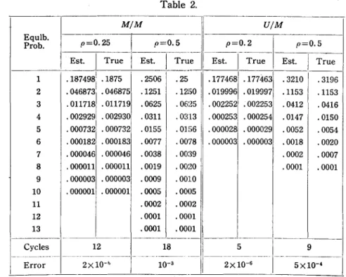
Table 2. ,---~---M/M U/M EquJh. p=0.25 p=0.5 Proh. I I p=0.2 p=0.5 -Est.

I

True Est.

I

Tr u e I Est.

_I

True Est.

I

True I 1 .187498' .1875 I .2506 .25 2 _{· 046873i • 046875} .1251 .12 3 .011718 .011719 .0625 .06 4 · 002929 . 002930 .0311 .03 5 · 0007321. 000732 .0155 .01 6 · 000182 .000183 .0077 .00 >0 I .177468 .1774631 .3210

I

.3196 .019996 .019997 .1153 .1153

~51

.002252 .002253 .0412 .0416 l3 .000253 .000254 .0147 .0150 i6 .000028 .000029 .0052 .0054 78 I .000003 .000003 .0018 .0020 7 .000046 .000046 .0038 .00 8 .000011 .000011 .0019 .00 19 1 .0002 .0007 lO .0001 .0001 9 .000003 .000003 .0009 .00 1 0 10 .000001 .000001 .0005 .00 )5 11 .0002 .00 )2 12 .0001 .00 n 13 .0001 .00 n -~----~----~--- - ---~-- -Cycles 12 18 5 9 --_ _ _ 0 _ _ 0 _ _ _ _ _ _ _ _ _ - ---~-- - - --- - - - -

(14)

106 Y. Tumura

(11-1) becomes smaller than the desirable number. The calculation will

'"

be completed by the adjustment -to satisfy (1. 1) or

L:

Pn

=

p.

u

3.3. Exemples. (1) M/ M/1 and U/ M/I. At first M/ M/I and U/ M/1

were calculated as a verification where U denotes the uniform distribu· tion A(,)=(;1/2),(0~,~2/;1) and =1(,>2/;1), since their true probabilities are known. The results are shown in Table 2. Table shows that for the adquate value of p (not so high) the convergence is pretty well.

(2) U/ U/l. The results are illustrated in Table 3 for p= 1/10, 1/5, 1/4, 1/3 and 1/2. p o 1 2 3 4 5 6 7 E{L} Table 3.

Equilibrium Probabilities of U/U/1 systems

0.1 0.2 0.25 1/3 0.5 1 , 1 '

-pi

q

plq

.9 .989639'.8 1.956841.75 1.930991.66667;.87189'.5

i'

67'70~

.096486 .010000'.185081.040001.22591'.062501• 28780. 111n!. 37942.24846 .003420 .0003511.01405.002981.02227. 0060l 040591 • 015181• 09679!. 06005 .000092 .0000091.00082.000171\.00170.000451.004471. 001651. 019481• 01185,

~

000002 .000000.00004.00000.00011.

ooool oood.

0001l 00355:. 002151 .00001 .000001•

ooool

00001 . 000621. 00038! .000111·00007i

i'

00002. 000011 .1036 .0107 .2158.0465.2760.0760.3843: 14711.

64951~

41;0-1 ----~ ~--- ~-I- --~---i

-:~~1----10~7--~

2X:0-' I 2X:O-' 2X:0-=-;'-1

-3~~0-'

i Acknowledgement

The author wishes to express his gratitude to Mr. K. Hayashi who has given valuable advice.

(15)

On the Equilibrium Probabilities of GI/G/l 101

REFERENCES

[ 1 J Takacs,' L, On the generalization of Erlang's formula, Acta Math. Acad. Sci. Hung., 7 (1956), 419-433.

[ 2 J -- -, On a queueing problem concerning telephon traffic, ibid., (1957), 8 325-335.

[ 3 J Tumura, Y., "Equilibrium equations method on generalized queuing Problems," T.R.U. Math., 3 (1967), 48-61.

On the Equilibrium Probabilities of GI/G/l