A Compact Encoding of Rooted Trees

全文

(1)Vol.2012-AL-138 No.4 2012/1/28. IPSJ SIG Technical Report. 1.564n+o(n) bits, where n is the number of vertices. Their method can be applied for rooted trees by specifying the root vertex with log n bits. The representation attains information-theoretically optimal bound by using auxiliary tables with o(n) space. Their result is theoretically nice, however the size of the tables would be huge. On the other hand, for unordered-rooted binary tree with n vertices, Iwata et al.[5] proposed a compact code with 1.4n + 4 bits without an auxiliary table. The information-theoretically optimal bound for such trees is 1.312n bits [2, 11]. Their result is near to the optimal length. Is there a coding scheme for rooted trees which attains information-theoretically optimal bound without an auxiliary table? In this paper, we design a coding method for rooted trees with n vertices without an auxiliary table. We experimentally show that an average length of our code is compact. For the case of n = 24, our method encodes a rooted trees into 1.556n bits per a rooted tree on average.. A Compact Encoding of Rooted Trees Katsuhisa Yamanaka†1 In this paper, we give compact codes for (unordered) rooted trees. We show that the codes are compact experimentally. For instance, the code occupies 1.556n bits per a rooted tree with n = 24 vertices on average. While an ordered tree of n vertices is encoded with 2n bits, which coincide with the information-theoretically optimal bound, our scheme is more compact.. 1. Introduction Trees are one of most important structures in computer science, and frequently used as models in various areas including searching, program parsing and mining semi-structured data such as XML. These days, we face a huge tree structure. In this paper we focus on a compact representation of an unordered tree. We design a binary code that represents an unordered tree compactly. For some class C, how many bits are needed to encode an element in C into a binary string S so that S can be decoded to reconstruct the original element? For any coding scheme the average length of S is at most log |C|⋆1 bits, which is called the information-theoretically optimal bound. 3 The number of ordered trees with n vertices is about c1 2n /n 2 , e.g. [10], where √ c1 = 1/4 π ≈ 0.1410. Hence the information-theoretically optimal bound is 2n bits (ignoring logarithmic terms). The number of rooted unordered trees 3 with n vertices is about c2 αn /n 2 , e.g. [10], where c2 = 0.5350 and α ≈ 2.9558. Hence, the information-theoretically optimal bound is 1.564n bits asymptotically (ignoring logarithmic terms). For ordered trees, there are many results on compact representations [1, 4, 6, 7]. For free trees, Farzan and Munro [3] proposed a succinct representation taking. 2. Definitions In this section, we give some definitions. Let G be a connected graph with n vertices. A path is a sequence of distinct vertices (v1 , v2 , . . . , vp ) such that (vi−1 , vi ) is an edge for i = 2, 3, . . . , p. The length of a path is the number of edges in the path. A tree is a connected graph with no cycle. A rooted tree is a tree with one vertex r chosen as its root vertex. For each vertex v in a rooted tree, let UP(v) be the unique path from v to r. The parent of v ̸= r is its neighbour on UP(v), and the ancestors of v ̸= r are the vertices on UP(v) except v. The parent of r and the ancestors of r are not defined. We say if v is the parent of u then u is a child of v, and if v is an ancestor of u then u is a descendant of v. A leaf is a vertex having no child. If a vertex is not a leaf, then it is called an inner vertex. The degree of a vertex v, denoted by d(v), is the number of children of v. An ordered tree is a rooted tree with a left-to-right ordering specified for the children of each vertex. We denote by T (v) the subtree of an ordered tree T consisting of a vertex v and all descendants of v that preserve the left-to-right ordering for the children of each vertex. Let CS(v) = (c1 , c2 , . . . , cd(v) ) be the. †1 Department of Electrical Engineering and Computer Science, Iwate University, Ueda 4-3-5, Morioka, Iwate 020-8550, Japan. [email protected] ⋆1 Log denotes logarithm to the base 2. 1. ⓒ 2012 Information Processing Society of Japan.

(2) Vol.2012-AL-138 No.4 2012/1/28. IPSJ SIG Technical Report. copies of v into the stack. We repeat this process for each vertex in preorder. 4. Canonical Representation of Rooted Trees. (a) Fig. 1. (b). Let R be a rooted tree. We can observe that R corresponds to many nonisomorphic ordered trees, since we can choose many left-to-right orderings for the children of each vertex in T . If we uniquely define a “canonical” ordered tree among ordered trees corresponding to R, then encoding canonical ordered trees means an algorithm that encodes rooted trees. This idea is also adopted for enumerating some classes of trees [8, 9]. However how to choose a canonical tree is slightly different from our method. Let T be an ordered tree with n vertices, and (v1 , v2 , . . . , vn ) be the list of the vertices of T in preorder. Then, a sequence DF (T ) = (d(v1 ), d(v2 ), . . . , d(vn )) is called the DF degree sequence of T . Let T1 and T2 be two ordered trees, and DF (T1 ) = (a1 , a2 , . . . , an ) and DF (T2 ) = (b1 , b2 , . . . , bm ) be their DF degree sequences. If either (1) ai = bi for each i = 1, 2, . . . , j − 1 and aj < bj , or (2) ai = bi for each i = 1, . . . , n and n < m, then we say that T1 is smaller than T2 , and write T1 ≺ T2 . For example, DF degree sequences of trees in Figs. 1(a), (b) and (c) are (3,3,2,0,0,0,0,1,1,0,2,0,0), (3,1,1,0,2,0,0,3,0,2,0,0,0) and (3,1,1,0,2,0,0,3,0,0,2,0,0), respectively. Now, we define a canonical representation of R as follows. The ordered tree T is a canonical tree of R if (1) T is isomorphic to R as a rooted tree and (2) DF (T ) is smallest among all ordered trees corresponding to R. For example, the ordered tree in Fig. 1(c) is the canonical tree, however the trees in Figs. 1(a) and (b) are not. We have the following two lemmas. Lemma 4.1 The canonical tree of a rooted tree is unique. Lemma 4.2 Let T be a canonical tree and CS(v) = (c1 , c2 , . . . , cd(v) ) be the child sequence for any inner vertex v of T . Then we have d(ci ) ≤ d(ci+1 ) for i = 1, 2, . . . , d(v) − 1. Proof. We assume otherwise for a contradiction. Let (v1 , v2 , . . . , vn ) be the sequence of vertices of T in preorder. We choose the minimum i such that CS(vi ) destroys the above condition. More precisely, i is the minimum (1 ≤ i ≤ n) such. (c). Three different ordered trees which are isomorphic as rooted tree.. sequence of the children of v from left-to-right. We call it the child sequence of v. Each ci is called the next sibling of ci−1 for i = 2, 3, . . . , d(v) and the previous sibling of ci+1 for i = 1, 2, . . . , d(v) − 1. Three trees in Fig. 1 are different ordered trees, but are isomorphic as rooted trees. 3. Depth-first Unary Degree Sequence In this section we briefly introduce a DFUDS (Depth-First Unary Degree Sequence) for an ordered tree [1]. DFUDS is a binary code for an ordered tree. It can represent an ordered tree with n vertices in 2n − 1 bits Let T be an ordered tree with n vertices, and v be a vertex of T . We define a block for v as follows. A block, denoted by B(v), for v is d(v) consecutive ‘0’s followed by one ‘1’. We traverse T with depth-first manner. If we visit v first, then output B(v). The obtained binary code is DFUDS for T . DFUDS consists of n blocks. The length of DFUDS is 2n − 1 bits, For instance, DFUDS for the tree in Fig. 1(a) is 00010001001110101100111. Decoding for DFUDS is a simple algorithm based on depth-first search of a tree using a stack. Here we carefully explain decoding for DFUDS, since it helps to understand how to decode our code explained later (Section 5). Let S1 be a DFUDS for an ordered tree. The first zero or more ‘0’s followed by one ‘1’ consist of the block for the root vertex r. By reading the first block, we know the degree d(r). For the block, we create a new vertex for r, then we push d(r) copies of r to a stack. Now, we explain how to decode vertices except r. We reconstruct each vertex in preorder. First we read a block B(v) consisting of d(v) ‘0’s followed by one ‘1’. Second we create a new vertex for v, then connect v to the vertex poped from the stack as the parent of v. Finally we push d(v). 2. ⓒ 2012 Information Processing Society of Japan.

(3) Vol.2012-AL-138 No.4 2012/1/28. IPSJ SIG Technical Report. that d(cj ) > d(cj+1 ) holds for some j in CS(vi ). If we exchange cj and cj+1 , then we obtain a smaller tree than T , which is a contradiction. □ We also have the following lemma. Lemma 4.3 An ordered tree T is canonical tree if T (u) ≺ T (v) or T (u) ∼ = T (v) for every u and its next sibling v. Proof. By contradiction. □. structures in a tree. ⋆1. .. Path Compression We give a formal definition of subpath. Let (v1 , v2 , . . . , vn ), (v1 ̸= r), be the sequence of vertices of T in preorder. A maximal subgraph induced by consecutive vertices vi , vi+1 , . . . , vj (i ≤ j) is an inner subpath if d(vk ) = 1 for k = i, i+1, . . . , j. During a depth-first search of T , if the current v has one child and the parent of v is not (or v is the root vertex with degree 1), then v may be the start vertex of an inner subpath in T . For such vertex, we store the length of the path starting from the child of v (or v) by an unary code. Now we explain our coding more formally. Assume that vi , vi+1 . . . , vj consist an inner subpath. After D(vi ), we encode a subpath vi+1 , . . . , vj of the inner subpath with j − i ‘0’s followed by one ‘1’. We can observe that vj+1 is a leaf or has two or more children. Then we encode vj+1 with ‘1’ if vj+1 is a leaf, otherwise with d(vj+1 ) − 1 ‘0’s followed by ‘1’. In B(vj+1 ), we can save one bits for a code of vj+1 if vj+1 has two or more children. However, if vi = vj , then we require one bit to represent a inner subpath with “length zero”. So, such case needs one more bit than S2 . We denoted by S3 obtained by adapting the above idea to S2 .. 5. Compact Codings and Decodings In this section we design compact codes for a rooted tree. Our idea is to encode the canonical tree of a rooted tree. If we encode the canonical tree of a rooted tree, then it also means that we can encode a rooted tree by Lemma 4.1. Given a rooted tree R, we construct a canonical tree T of R, then we encode a canonical tree with a binary code. The obtained code is the code for R. Our encoding method is based on DFUDS for an ordered tree. By modifying DFUDS, we design a compact code for a canonical tree. In this section, we introduce three ideas for improvements. From now on, we denote by S1 DFUDS for T . Difference The first idea for improvements is to store the number of children of each vertex as a difference from its previous sibling. Let u, v be a vertex and its previous sibling. A difference block D(u) is equal to B(u) if u is the first child of its parent, and D(u) is a code consisting of d(u) − d(v) ‘0’s followed by ‘1’ if u is not the first child of its parent. We define S2 a binary code obtained by arranging all difference blocks in preorder of vertices. Decoding the original rooted tree from S2 is almost same as decoding of DFUDS. If the first i vertices in preorder are decoded, then we can compute d(vi+1 ) from D(vi+1 ), which is (i + 1)the block in S2 , and the degree of the previous sibling of vi+1 . Therefore we can decode S2 . Now we estimate the length of S2 . Clearly we have |S0 | ≤ |S1 |. Are there trees that satisfy |S0 | = |S1 |? For instance, if T is a path, S2 needs 2n − 1 bits. So we can observe that, if T includes many paths as its subgraphs, then |S2 | comes up to |S1 |. From this observation, we have an idea which is to compress path. Saving for Root Edges and Right Leaves The last idea is as follows. Let r be the root vertex of T . If we omit D(r) in ′ S1 (similarly S2 and S3 ), S1 represents “d(r) trees”. Let S1 be a code obtained by omitting D(r) in S1 . By the decoding of S1 , we can obtain d(r) trees from ′ S1 . Then we insert the root vertex with an edge to each tree. The resulting tree is T . In addition, we can omit blocks for “right” leaves. A vertex v is the rightmost vertex of T if v is the last vertex in preorder. Let v be the rightmost vertex of T , and assume that the parent of v is not r. All the siblings of v are leaves. A leaf ℓ is right leaf if ℓ is the rightmost vertex or ℓ is a sibling of the rightmost vertex. Since the number of right leaves can be compute ⋆1 If T is a star, S2 satisfies 2n − 1 bits too. However, in our coding, we focus on compressing a path structure.. 3. ⓒ 2012 Information Processing Society of Japan.

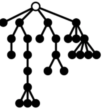
(4) Vol.2012-AL-138 No.4 2012/1/28. IPSJ SIG Technical Report. Fig. 2. An environment for our experiment is as follows. (1) OS: FreeBSD 8.2RELEASE, (2) CPU: AMD Phenom(tm) II X6 1065T Processor (2909.62-MHz K8-class CPU), (3) Main memory: 4GB and (4) Programming language: C. Table 1 shows the average length of each code per a rooted tree with n vertices. Each column means S1 (DFUDS), S2 (DFUDS + difference), S3 (DFUDS + difference + path compression), S4 (DFUDS + difference + saving root edges and right leaves) and S5 (DFUDS + difference + path compression + saving root edges and right leaves), respectively. “Optimal” means the optimal average length of a code. Let Tn be a set of rooted trees with n vertices. The optimal average length per tree can be obtained by calculating log |Tn |. For instance, for n = 24, S4 needs 1.556n bits per a rooted tree with 24 vertices on the average. This also means S4 needs 1.556 bits per a vertex in a rooted tree with 24 vertices. Since there is only one tree with n vertices for n = 1 or n = 2, we did not deal with the two cases here. In this experiment, first, we enumerate all canonical trees with n vertices, then encode all the trees by each coding method, and then we calculate the average length of each code per tree. All factors in Table 1 are plotted in Fig. 3 for each code. Fig. 3 shows that S4 is the most compact among our codes. Comparing S4 with the optimal length of code, S4 is near to the optimal length. S4 needs 1.556n bits per a rooted tree with n = 24 vertices on the average, and the optimal average length of code is 1.228n bits for the same tree. So, we conclude that S4 is a compact code from this experimental results. Unfortunately, path compression did not improve the average length. The two codes S3 , S5 which perform path compressions are slightly larger than S2 and S4 , respectively.. A canonical tree for examples.. from the block for the parent of v, we can omit blocks for the right leaves. Note that if v is a child of r, we cannot omit. Also we can save the last ‘1’, which is the last ‘1’ in the block for the parent of v, in the code, since the last bit is always ‘1’. This idea can be adopted even if the parent of v is the root. We denoted by S4 and S5 obtained by omitting root edges, right leaves and the last ‘1’ in S2 and S3 , respectively. Examples For example, S1 , S2 , S3 , S4 and S5 for the canonical tree in Fig. 2 are: S1 = 000011001011010101000111100110100111000111000011111, S2 = 0000110010111010100011111101001110111000011111, S3 = 00001100101111001011111101101110111000011111, S4 = 100101110101000111111010011101110000, S5 = 1001011110010111111011011101110000. We have the following theorem. Theorem 5.1 We can encode a canonical tree with S1 , S2 , S3 , S4 , S5 in O(n) time, and a decoding for each code can be done in O(n) time using a stack.. 7. Conclusion We have designed four new codes for a rooted tree. By coding canonical trees, we designed codes for (unordered) rooted trees. Our codes are based on DFUDS [1] which is a codes for an ordered tree. By improving DFUDS, we propose compact code for a rooted tree. Then, we have shown that our codes are compact by experiments.. 6. Experimental Results In this section, we show experimental results of the five codes S1 , S2 , S3 , S4 and S5 explained in the previous section.. 4. ⓒ 2012 Information Processing Society of Japan.

(5) Vol.2012-AL-138 No.4 2012/1/28. IPSJ SIG Technical Report. Table 1. 2. |S1 |. |S2 |. |S3 |. |S4 |. |S5 |. Optimal. (bits/tree). (bits/tree). (bits/tree). (bits/tree). (bits/tree). (bits/tree). 1.667n 1.750n 1.800n 1.833n 1.857n 1.875n 1.889n 1.900n 1.909n 1.917n 1.923n 1.929n 1.933n 1.938n 1.941n 1.944n 1.947n 1.950n 1.952n 1.955n 1.957n 1.958n. 1.667n 1.750n 1.778n 1.800n 1.804n 1.810n 1.811n 1.812n 1.812n 1.812n 1.812n 1.811n 1.811n 1.810n 1.810n 1.809n 1.809n 1.809n 1.808n 1.808n 1.807n 1.807n. 1.667n 1.750n 1.800n 1.817n 1.821n 1.826n 1.827n 1.827n 1.827n 1.827n 1.826n 1.826n 1.825n 1.824n 1.824n 1.823n 1.823n 1.822n 1.822n 1.821n 1.821n 1.820n. 0.333n 0.562n 0.733n 0.883n 0.994n 1.090n 1.164n 1.226n 1.277n 1.320n 1.356n 1.387n 1.414n 1.437n 1.458n 1.477n 1.493n 1.508n 1.522n 1.534n 1.545n 1.556n. 0.500n 0.625n 0.800n 0.933n 1.039n 1.128n 1.199n 1.258n 1.306n 1.347n 1.382n 1.412n 1.437n 1.460n 1.480n 1.498n 1.514n 1.529n 1.542n 1.554n 1.564n 1.574n. 0.333n 0.500n 0.634n 0.720n 0.798n 0.856n 0.907n 0.949n 0.986n 1.018n 1.047n 1.072n 1.095n 1.115n 1.134n 1.151n 1.166n 1.181n 1.194n 1.206n 1.217n 1.228n. 1.8 1.6. The factor of bitsize per tree. # of vertices n=1 n=2 n=3 n=4 n=5 n=6 n=7 n=8 n=9 n = 10 n = 11 n = 12 n = 13 n = 14 n = 15 n = 16 n = 17 n = 18 n = 19 n = 20 n = 21 n = 22 n = 23 n = 24. 1.4 1.2 1 0.8 0.6 0.4. S1: DFUDS S2: DFUDS + difference S3: DFUDS + difference + path compression S4: DFUDS + difference + saving root edges and right leaves S5: DFUDS + difference + path compression + saving root edges and right leaves Optimal. 0.2 0 0. 5. Fig. 3. 10 15 The number of vertices. 20. 25. The average lengths of each code.. The experimental results show that S4 is compact, but the optimal average length seems to be properly smaller than the average length of S4 . So, we want to know asymptotic behaviors of the two length. The optimal average length converges 1.564n bits asymptotically. Now, how many bits are required for S4 asymptotically? Other future tasks are to (1) design a more compact code for a rooted tree, and (2) design compact codes for other graph classes so that it attains (or is near to) the information-theoretically optimal bounds without an auxiliary table.. The average lengths of our codes. S1 : DFUDS, S2 : DFUDS + difference, S3 : DFUDS + difference + path compression, S4 : DFUDS + difference + saving root edges and right leaves, S5 : DFUDS + difference + path compression + saving root edges and right leaves.. References [1] D. Benoit, E. Demaine, J. Munro, and V. Raman. Representing trees of higher degree. Algorithmica, 43:275–292, 2005. [2] I.Etherington. Non-associate powers and a functional equation. The Mathematical. 5. ⓒ 2012 Information Processing Society of Japan.

(6) Vol.2012-AL-138 No.4 2012/1/28. IPSJ SIG Technical Report. Gazette, 21:36–39, 1937. [3] A. Farzan and J. Munro. A uniform approach towards succinct representation of trees. In Proc. of the 11th Scandinavian workshop on Algorithm Theory (SWAT2008), volume 790 of Lecture Notes in Computer Science, pages 173–184, 2008. [4] R. Geary, R. Raman, and V. Raman. Succinct ordinal trees with level-ancestor queries. ACM Transactions on Algorithms, 2(4):510–534, 2006. [5] K. Iwata, S. Ishiwata, and S. Nakano. A compact encoding of unordered binary trees. In Proc. of the 8th Annual Conference, Theory and Applications of Models of Computation, volume 6648 of Lecture Notes in Computer Science, pages 106–113, 2011. [6] G.Jacobson. Space-efficient static trees and graphs. Proc. of the 30th IEEE Symposium on Foundations of Computer Science, (FOCS1989), pages 549–554, 1989. [7] J.Munro and V.Raman. Succinct representation of balanced parentheses and static trees. SIAM Journal on Computing, 31(3):762–776, 2001. [8] S.Nakano and T.Uno. Constant time generation of trees with specified diameter. Proc. the 30th Workshop on Graph-Theoretic Concepts in Computer Science, (WG 2004), LNCS 3353:33–45, 2004. [9] S. Nakano and T. Uno. Generating colored trees. Proc. the 31th Workshop on Graph-Theoretic Concepts in Computer Science, (WG 2005), LNCS 3787:249–260, 2005. [10] R.Sedgewick and P.Flajolet. An introduction to the analysis of algorithms. Addison Wesley, 1996. [11] J. Wedderburn. The functional equation g(x2 ) = 2α + [g(x)]2 . The Annals of Mathematics, Series 2, 1937.. 6. ⓒ 2012 Information Processing Society of Japan.

(7)