Panel Data Research Center at Keio University
DISCUSSION PAPER SERIES
DP2016-001 April, 2016
Economic and Time Constraints on Women’s Marriage, Childbirth and Employment, and Effects of Work-Life Balance Policies
Empirical Analysis Using Japanese Household Panel Surveys Yoshio Higuchi*
Kazuyasu Sakamoto** Risa Hagiwara***
【Abstract】
This paper investigates the effects of economic and time constraints on women’s marriage, childbirth, and employment. According to our analyses using household panel surveys, we find the following. (1)Women who graduated from college and live with their parents or their spouse’s parents have a high likelihood of marriage. Women in full-time employment and those earning a high hourly wage tend to get married. Regular employees whose working hours and commuting times are short tend to get married. (2) In regard to continued employment after marriage, the husband’s income has negative effects but the wife’s hourly wage rate has positive effects on continued female employment. Women who can easily take childcare leave tend to continue working. (3) The likelihood of childbirth increases with the husband’s time spent on housework and childcare. (4) A higher husband’s income discourages the wife’s continued employment after childbirth, but women earning a higher hourly wage rate are more likely to continue working after giving birth. In addition, the likelihood of continued employment after childbirth is higher among women in regular employment compared with non-regular employment. Long working hours and long commuting times discourage women from continuing to work after childbirth, while childcare leave and the availability of childcare facilities have positive effects. (5) The more time the husband spends on housework and childcare, the more likely the wife is to return to work after childbirth, though the wife is less likely to do so when the husband’s income is higher. Focusing on differences between birth cohorts of women, young cohorts are significantly less likely to likely to get married but are more likely to continue working, even when
holding equal the above-mentioned economic and time constraints and support for work-life balance. The likelihood of continued regular employment after childbirth is high in young cohorts. However, the likelihood of continued non-regular employment is low among non-regular employees in the young cohorts.
*Professor, Faculty of Business and Commerce, Keio University
**Associate Professor, Faculty of Social and Information Studies, Gunma University ***Lecturer, Department of Economics, Meikai University
Panel Data Research Center at Keio University
Keio University
Economic and Time Constraints on Women’s Marriage, Childbirth
and Employment, and Effects of Work-Life Balance Policies
*Empirical Analysis Using Japanese Household Panel Surveys
Yoshio Higuchi
※1Kazuyasu Sakamoto
※2Risa Hagiwara
※3Abstract
This paper investigates the effects of economic and time constraints on women’s marriage, childbirth, and employment. According to our analyses using household panel surveys, we find the following. (1)Women who graduated from college and live with their parents or their spouse’s parents have a high likelihood of marriage. Women in full-time employment and those earning a high hourly wage tend to get married. Regular employees whose working hours and commuting times are short tend to get married. (2) In regard to continued employment after marriage, the husband’s income has negative effects but the wife’s hourly wage rate has positive effects on continued female employment. Women who can easily take childcare leave tend to continue working. (3) The likelihood of childbirth increases with the husband’s time spent on housework and childcare. (4) A higher husband’s income discourages the wife’s continued employment after childbirth, but women earning a higher hourly wage rate are more likely to continue working after giving birth. In addition, the likelihood of continued employment after childbirth is higher among women in regular employment compared with non-regular employment. Long working hours and long commuting times discourage women from continuing to work after childbirth, while childcare leave and the availability of childcare facilities have positive effects. (5) The more time the husband spends on housework and childcare, the more likely the wife is to return to work after childbirth, though the wife is less likely to do so when the husband’s income is higher. Focusing on differences between birth cohorts of women, young cohorts are significantly less likely to likely to get married but are more likely to continue working, even when holding equal the above-mentioned economic and time constraints and support for work-life balance. The likelihood of continued regular employment after childbirth is high in young cohorts. However, the likelihood of continued non-regular employment is low among non-regular employees in the young cohorts.
Key words:
marriage, childbirth, continued employment, reemployment
* This research used data from the Ministry of Health, Labour and Welfare’s Longitudinal Survey of Adults in the 21st Century and the Japanese Panel Survey of Consumers by the Institute for Research on Household Economics. We would like to express our sincere gratitude to the Ministry of Health, Labour and Welfare and the Institute for Research on Household Economics for supplying the data. This research was supported by a Grant-in-Aid for Scientific Research (2014, policy, general 003) from the Ministry of Health, Labour and Welfare and by the Japan Society for the Promotion of Science under the research theme “Multi-Dimensional Dynamic Analysis of Gender Equality and the Role of the Family in Internationally Comparable Data” as part of the Topic Setting Program to Advance Cutting-Edge Humanities and Social Science Research. Any errors in this report are the responsibility of the authors alone.
※1 Professor, Faculty of Business and Commerce, Keio University
※2 Associate Professor, Faculty of Social and Information Studies, Gunma University ※3 Lecturer, Department of Economics, Meikai University
1
1. Introduction
For women, getting married and having children incurs heavy costs: It limits the amount of time women are able to use for themselves and constrains their degrees of freedom. If various constraints prevent women from marrying, having children, or continuing to work despite their desire to do so, in many cases they will give up on these things. For women, what sorts of factors affect marriage, having children, and continuing to work or reentering the workforce? According to economic theory, women will choose whether to get married, have children or work after comparing expected costs and benefits. But what factors constitute these costs and benefits and what impact does each have? In this paper, we focus on economic and time constraints. We use household panel surveys, which track the same individuals over an extended time period, to conduct empirical analysis on the impact of policy measures for easing constraints on marriage and childbirth, employment continuity, and reentry to the workforce. By investigating differences among birth cohorts that remain after controlling for financial and time constraints, we aim to uncover unspecified (including psychological) factors that affect hopes and benefits regarding marriage, childbirth, childcare, and employment such as education, family environment, and societal environment.
Before moving to our empirical analyses, we first give an overview of recent changes surrounding women’s marriage, childbirth, and employment using public statistics. The marriage rate In Japan started declining in 1973, around the time of the first oil shock. After showing slight increases or level trends from 1988 through 2010, the rate has declined since 2010, albeit marginally. Over this period, there has been a steady increase in the age at marriage. Meanwhile, the total fertility rate, which was over 4 immediately after the Second World War, has declined markedly thereafter. From the mid-1950s through the time of the first oil shock, total fertility rate was roughly flat, before again starting to decline, and in 2005 it reached a record low of 1.26 and has recovered slightly to 1.43 today. However, this is largely due to an increase in fertility rates among women in their 30s. Due to the shrinking number of women in their 20s and 30s, the number of babies born each year is on a declining trend. (According to preliminary figures for 2015, the number of births rose from the prior year, albeit only slightly.) Meanwhile, employment rates for women have been rising recently. According to the Labour Force Survey by the Ministry of Internal Affairs and Communications, there has been an across-the-board increase in female employment rates from 1994 to 2014. This was particularly notable in women aged 25-29 and 30-34 years, which rose by 14.0 percentage points (pp) and 16.0 pp respectively. A plot of female employment rate versus age traces an M-shaped curve, and its low point has increased markedly. Nonetheless, as before, from the late 20s through the 30s, there remains a large decline of roughly 8 pp in the female employment rate (Figure 1).
The National Fertility Survey by the National Institute of Population and Social Security Research shows how employment patterns have changed for women around the time of major life events. According to this survey, the percentage of women who keep working around the
time of marriage rose by 4.4 pp from the late 1980s to the late 2000s, and the percentage of women quitting employment upon marriage has declined by 11.7 pp (Figure 2). The number of women continuing to work after marriage is gradually increasing. Next, we examine employment trends around the time of birth of the first child. As mentioned previously, the number of women quitting their jobs when they get married has declined, so the share of women not working before pregnancy has fallen by 11.4 pp. However, the share of women quitting employment due to childbirth has increased by 6.5 pp, so there has consequently not been any major change in the share of women continuing to work. The aggregate percentage of women continuing work after the birth of their first child (the sum of those who take and do not take childcare leave) remains stuck at around 27%.
To facilitate continued employment of women after life events, the government has established proactive measures under the Equal Employment Act and revised the Child Care and Family Care Leave Act. Companies, too, have taken a number of initiatives. Higuchi (2007) notes a steady improvement in employment continuity due to the launch of government initiatives to support women and the improved operation of existing schemes. Yet, even today, there are no signs of an end to women withdrawing from the labor market after a life event. The tendency remains that after the burden of childcare has eased somewhat, they reenter the workforce as part-time employees. This is not just a matter of making better use of female labor to augment the workforce as the working age population in Japan declines. In light of the large gap that remains between the percentage of women who want to work and actual employment rates, putting in place the social infrastructure so that women can build their own careers while having and raising children is an important issue in itself.
What sorts of factors are driving these changing circumstances? Why are the desired changes not progressing much? Below, we elucidate these issues, using panel data from tracking surveys of the same individuals with further comparisons of differences among cohorts. This paper is structured as follows. In Section 2, we review previous research analyzing women’s marriage, childbirth, and employment. In Section 3, we review the data used in this research. Section 4 presents the results of analyzing women’s marriage decisions and Section 5 shows results of our analysis of changes in women’s employment after marriage. Section 6 presents an analysis of childbirth decisions, and Section 7 shows the results of analyzing changes in employment after childbirth. Section 8 reviews estimation results for women reentering the workforce. The final section presents the conclusions of this research.
Figure 1. Female employment rates by age group (1994 vs. 2014)
Source: Ministry of Internal Affairs and Communications, Labour Force Survey
Figure 2. Changes in wife’s employment status after birth of the first child by year of marriage
Source: National Institute of Population and Social Security Research (2011) 14th National Fertility Survey: Marriage and Fertility in Japan, Figure 5-2, 5-3
15.8 70.5 61.7 51.4 60.1 68.3 69.8 66.3 55.4 38.6 15.8 15.6 65.8 75.7 68.0 68.3 71.8 74.4 73.4 66.3 47.6 14.3 0 10 20 30 40 50 60 70 80 15-19 20-24 25-29 30-34 35-39 40-44 45-49 50-54 55-59 60-64 over 65 1994 2014 % 5.7 8.1 11.2 14.8 17.1 18.3 16.3 13 11.9 9.7 37.4 37.7 39.3 40.6 43.9 35.5 34.6 32.8 28.5 24.1 3.1 3.4 3.8 4.1 5.2 0% 10% 20% 30% 40% 50% 60% 70% 80% 90% 100% 1985-89 1990-94 1995-99 2000-04 2005-09 No details
Unemployed before pregnancy Quit after childbirth
Kept working (no childcare leave) Kept working (used childcare leave)
56.6 56.9 58.3 62.4 61 37.3 34.5 31.2 25.6 25.6 1.1 1.0 1.2 1.2 1.5 2.9 4.1 5.8 7.3 7.7 2.0 3.6 3.6 3.4 4.2 0% 10% 20% 30% 40% 50% 60% 70% 80% 90% 100% 1985-89 1990-94 1995-99 2000-04 2005-09 No details
Unemployed before marriage Employed after marriage Quit when married Continued employment
2. Previous research
Since panel data became available, there have been many studies analyzing employment changes around the times of marriage and childbirth, starting with Higuchi (2000). Many of these studies analyze the combined effects of work related initiatives such as those for childcare leave, flextime, and reduced working hours, as well as childcare facilities and the husband’s participation in housework and childcare (time). In this section, we review previous literature, grouping it into research that uncovers positive effects and research that uncovers negative effects.
First is taking childcare leave. Higuchi (1994), Higuchi et al. (1997), Morita and Kaneko (1998), Shigeno and Okusa (1998), Wakisaka (2002), Suruga and Zhang (2003), and Noguchi and Shimizutani (2004) report that providing childcare leave results in higher rates of employment continuity after childbirth. Toda (2012) uses the same the Longitudinal Survey of Adults in the 21st Century as our research does and examines the impacts of work-life balance support measures such as childcare leave on marriage, childbirth, and employment continuity. This work confirms that childcare leave measures promote continued employment after childbirth. Further, several studies find an effect on women’s employment continuity of providing childcare facilities (Shigeno and Okusa,1999; Nagase, 2003; Higuchi et al., 2007). Some research examines the impact on childbirth and marriage (Suruga and Nishimoto, 2002; Suruga and Zhang, 2003; Shigeno and Matsuura, 2003); Shigeno, 2006). These studies show that childcare leave promotes childbirth. Shimizutani and Noguchi (2004) point out that benefit programs at the workplace in addition to childcare leave, such as flextime systems, shorter working hours, and in-house childcare facilities promote the participation of married women in the workforce. Further, with regard to childbirth, Suruga and Nishimoto (2002) note that childcare leave, promotions during childcare leave, guarantees of promotion and pay upon returning to work, measures to maintain and improve employee skills, and measures to enable staggered starting and finishing times promote fertility. Noguchi (2011) reports that company measures to support childcare facility use, telecommuting, geographically limited work, and systems to reemploy workers who have quit to marry or give birth promote fertility. Research by Yoshida and Mizuochi (2005) suggests that higher capacity at authorized childcare facilities encourages the birth of a second child. Regarding the impact of the husband’s housework and childcare activity on the wife’s participation in the workforce and childbirth, Koba et al. (2009) find that these factors increase the wife’s propensity to have children. Yamagami (1999) reports that the more the husband helps with housework and childcare, the greater the probability that the wife will work. Mizuochi (2006) points out that the significance of the husband’s participation in childcare differs depending on whether the wife’s employment status is viewed endogenously or exogenously. An analysis by Nakano (2009), taking into consideration this endogeneity, shows a clear impact whereby the husband’s participation in housework and childcare promotes the wife’s employment.
Conversely, other research finds no significant impact of work-related measures such as childcare leave, flextime, and shorter working hours, or of childcare facilities and the husband’s participation (time) in housework and childcare, or at best the impact is marginally significant.
Shigeno and Okusa (2001), Sakatsume and Kawaguchi (2007), and Noguchi (2011) examine the effect of childcare leave. There is also research on marriage: According to Shigeno and Okusa (1998), childcare leave has no impact on marriage. Specifically, research using macroeconomic statistics and cohort data comparing periods before and after the introduction of childcare leave finds that it has only a small impact on continuing employment (Shigeno and Okusa, 1998; Nagase, 1999; Iwasawa, 2004; Imada and Ikeda, 2006; Shikata and Ma, 2006; Saito and Ma, 2008; Suga, 2011; Unayama, 2011). According to Suga (2011), since the promotion of childcare leave and other measures began in order to stem the decline in the birth rate, the younger generation of women has shifted the timing of quitting their pre-marriage work from around the time of the marriage to after their first pregnancy. However, the share of women that are still working one year after giving birth has not shown any notable increase. In the young cohorts, the likelihood of women quitting work during their first pregnancy is particularly high. Unayama (2011) points out that the rate of women quitting work due to marriage and pregnancy was 86.3% from 1980-2005, and that since 1980 it has not changed regardless of the age at marriage. Further, while the provision of childcare facilities reduces the percentage of women who quit work, childcare leave and living with parents have no significant impact on employment separation rates. Senda (2002) reports that childcare facilities have no impact on women continuing to work, at least in the major metropolitan centers of Japan. Yoshida and Mizuochi (2005) report that the capacity of authorized childcare centers has no significant impact on women’s workforce participation. According to Asai et al. (2015), after controlling for specific prefectural effects (e.g., traditional values), the correlation disappears between the availability of public childcare services and employment rates. Suruga (2011) notes that the husband’s housework hours have no impact on the wife’s desire to have children: and that although it is thought that the husband will increase the time allocated to housework if his working hours and commuting time become shorter, thus facilitating the wife’s employment, there is no impact on increasing regular employment. There is a plethora of research regarding employment changes relating to women’s marriage and fertility, but the results are not necessarily consistent.
The estimation results of much previous research suggest that few women with high levels of education find new employment after quitting work to get married or have children (Higuchi, 2000; Hirao, 2005; Sakamoto, 2009). These results are interpreted as follows. Higher educational attainment among women results in a stronger tendency to be oriented toward intrinsic rewards—women want their knowledge and experience to be put to use in a job that is challenging and gives a feeling of accomplishment (Japan Institute of Labour, 2000; Takeishi, 2001). However, either because job openings in the labor market do not meet such criteria, or because their schooling took so long, these women are late in marrying and having their first child. When they are ready to reenter the workforce once the childcare burden is lighter, they are able to choose from only a limited number of potential jobs. This is the job opening-job seeker mismatch hypothesis. Further, considering the tendency for women to marry someone of equal or higher socioeconomic status, highly educated women have a greater likelihood of having a spouse who is highly educated and earning a high salary, so women’s motivation to earn an income after marriage will not be as strong (weak income motivation hypothesis). According to Hirao (2005), for female college graduates in particular, there is a strong effect of
husband’s income on wife’s reemployment. These results regarding the employment of married women are in line with the first Douglas-Arisawa Law: When the main breadwinner has a high salary, other household members have low employment rates (Higuchi, 1995; Wakisaka and Tomita, 2001).
It is thought that the timing of women’s return to the workforce depends on when their children become independent. However, detailed research into the careers of 19 women over the age of 35 years via interview surveys by the Japan Institute for Labour Policy and Training (2006) finds wide discrepancies in the timing of returning to work. For some women, it was before the first child had entered elementary school and for some it was not until the youngest child had entered high school (Okutsu, 2006); the timing depends on the women’s own way of thinking. Sakamoto (2012) hypothesizes a gendered division of labor attitudes behind the decision not to continue work or not to return to work. The idea is that women’s ways of thinking govern their employment decisions and they think that the spouses should specialize: the wife should work inside the home, doing housework and raising the children, while the husband should participate in the labor market to earn an income. Further, Nakamura (2010) points out that women’s career goals are discernible before women enter the workforce, at the time of university enrollment. If female students enroll at vocational or liberal arts colleges or colleges with elements of both, this has a major bearing on where they subsequently find employment, as well as their working careers.
Compared with previous research, our research makes three key advances. First, it uses panel data. This makes it possible to directly track work changes due to marriage and childbirth for the same individuals. Second, this research comprehensively analyzes the women themselves regarding commuting time, wages, husband’s income, childcare services, and the time that the husband devotes to housework and childcare. Almost all the analyses in previous research focus on a single factor. There has been little comparative analysis of multiple factors to examine which have the biggest impact. Third, the present research examines cohort differences. As explained below, the Longitudinal Survey of Adults in the 21st Century available for this research spanned 2002-2011, so it was possible to analyze only a single cohort. However, the Japanese Panel Survey of Consumers has had cohorts added several times since 1993. This enables analysis of three different birth cohorts in 10-year intervals and the analysis of differences among the cohorts.
3. Data
In this research, we analyze the Ministry of Health, Labour and Welfare’s Longitudinal Survey of Adults in the 21st Century and the Japanese Panel Survey of Consumers by the Institute for Research on Household Economics. We also employ official statistics (including the Employment Status Survey and the National Fertility Survey) to supplement these panel data surveys on women’s employment and perform analysis in line with our aforementioned goals. The Ministry of Health, Labour and Welfare’s Longitudinal Survey of Adults in the 21st Century covers men and women who were aged 20-34 years as of the end of October 2002, selected
from across Japan. The survey consists of two waves: those who were adults in 2002 and those were adults in 2012. However, only data for the 2002 wave could be used in this research, so we have been unable to analyze intergenerational differences. There are two benefits from using these data. First, respondents are obliged to answer because these are official government statistics, so there is a higher response rate and a large sample size in both time-series and cross-sectional data1. Second, the Longitudinal Survey of Adults in the 21st Century includes variables that enable the identification of region (prefecture), allowing matching of information that indicates regional characteristics such as the availability of childcare facilities. However, a shortcoming is that there are a limited number of question items because the survey is for official statistics; there are fewer questions than in the panel data collected by universities and research institutes.
In this research, we use regional information from the Longitudinal Survey of Adults in the 21st Century integrated with data from the Ministry of Health, Labour and Welfare’s Survey of Social Welfare Institutions. Using this survey and population estimates from the Ministry of Internal Affairs and Communications, we estimate “underlying capacity” as defined by Unayama (2011), based on the female population aged 25-34 years and childcare facilities, and we then use this in our analysis. Research prior to Unayama (2011) used childcare facility waiting lists and childcare facility capacity, but as Unayama (2011) pointed out, these cannot be considered appropriate for showing the availability of childcare facilities because the number of children resulting from marriage and childbirth affect these indicators. For example, even if childcare facilities were insufficient, if marriages and births were declining, then the indicators would improve and lead to problems such that the provision of childcare facilities would be overestimated. Conversely, even if childcare facilities were to increase, if the number of people desiring places also increased as a result, the number of children on waiting lists would tend to increase. Therefore, in this research, to get an indication of underlying childcare demand, including from those not yet married, we use “underlying capacity.” Note that in this paper we refer to this underlying capacity as “childcare facility capacity.” Further, as an indicator of regional labor supply and demand we use the Ministry of Health, Labour and Welfare’s job-offers-to-applicants ratio from the ministry’s job and employment placement service statistics (general employment placement situation) in our estimation.
The Japanese Panel Survey of Consumers by the Institute for Research on Household Economics started with women who were aged 24-34 years in September 1993 (and men who were their spouses). Its key characteristics are that many of the questions are aimed at women and that the survey has been conducted over a long period of time. This continuous survey has been conducted for over 20 years, and the initial cohort is now aged 45-55 years. It thus covers not just marriage and childbirth, but subsequent other life events. Further, new respondents were included as additional samples: women aged 24-27 years in 1997; 24-29 years in 2003; 24-28 years in 2008; and 24-28 years in 2013. The survey has the advantage of following intergenerational differences. Our research exploits the length of the survey period, and uses the data primarily to analyze reemployment. Further, we show estimation results for birth cohort 1 However, survey items that needed to be answered by filling in a number such as salary did not necessarily have a high response rate.
8
dummies (with those born in the 1960s as the reference group for those born in the 1970s and 1980s). This was to capture the effects of age on marriage and childbirth decisions, and continued employment after marriage or childbirth. From the next section onward, using the data discussed, we show the results of analyzing marriage and childbirth decisions and changes in employment status after marriage or childbirth as well as reemployment after childbirth. 4. Marriage decisions
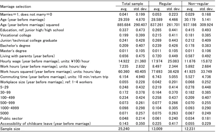
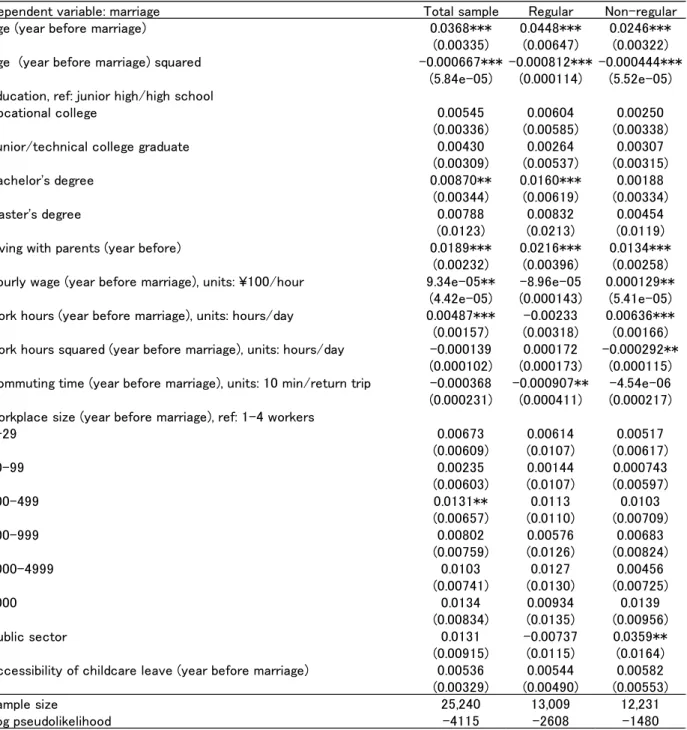
In this section, we use the Longitudinal Survey of Adults in the 21st Century to examine which factors have affected marriage decisions since the start of the 2000s. Table 1 shows descriptive statistics for the sample used in marriage decision estimates. Table 2 shows the results of panel probit analysis of the data sample in Table 1. We restricted the analysis sample to women who had not been married the previous year, and the dependent variable took a value of 1 for women who had married by the next year and 0 for those who had not yet married. In addition to basic attributes such as age and education, we used various data concerning the workplace in the previous year as explanatory variables.
From Table 2 we can see the following. First, among individual attributes, age and age squared show positive and negative signs respectively, and are significant. As age increases the number of women who marry increases, although growth tapers off. Looking at the education dummy, compared with junior high and high school graduates, college graduates have higher marriage rates (+0.87%). For the living-with-parents2 variable, there was a significant positive effect in all cases (+1.34% to +2.16%). The results are diametrically opposed to part of the “parasite single” hypothesis proposed by Prof. Masahiro Yamada in the 1990s. Yamada asserted that living with high-income parents was very comfortable for unmarried persons whose parents would pay housing and living expenses, as the singles could enjoy a lavish lifestyle. Therefore, they would not choose marriage because living together with a spouse whose income was lower than their parents would mean that they would be deprived of free time and their luxurious lifestyle. Below are conceivable explanations as to why our results differ. First is that singles living with their parents did not necessarily live a “lavish single lifestyle” since the late 1990s due to the economic recession. Since the economic downturn of the 1990s, those in their 20s experienced hardship during the recession, and in an increasing number of cases,” their first job was non-regular employment such as part-time or casual work. They would not be able to achieve economic independence if they left the family home and so they remained there in an increasing number of cases (Kitamura and Sakamoto, 2004; Nishi, 2010). Further, their parent’s generation was not as well off as before, so in an increasing number of households having the children live with them enabled both sides to support each other’s lifestyles (Kitamura and Sakamoto, 2007). From these facts, it is clear that singles living with their parents were not in a position to enjoy one-sided benefits of basic living conditions; they had responsibilities as a member of the household. Further, when the parents started retiring, the children had to take up the household 2 The living-with-parents dummy was a binary variable set at 1 if the respondent lived with their or their spouse’s parent(s) and 0 if they did not. The form for the Longitudinal Survey of Adults in the 21st Century, instructs respondents to answer “living together” if the buildings are separate but on the same grounds. Therefore, “living together” means “living in the same building” or “living on the same grounds” in this research.
9
responsibilities in their stead and had to do the daily cooking and household chores and ultimately needed to look after the parents. It is conceivable that living in the family home was a factor pushing them to choose marriage.
We next look at the impact of work-related factors. Commuting times (in the previous year) for regular employees had a negative and significant impact (-0.09% for every 10 min). For non-regular employees, too, commuting times had a negative sign, though it was not significant. From this, we confirmed that longer commuting times decreased marriage rates. Commuting times not only have a fundamentally negative impact on life satisfaction (Asano and Kenjoh, 2011), but also cut into the time available to socialize or engage in hobbies, a conceivable reason that workers may not have time to pursue romantic interests.
Meanwhile, looking at working hours and the squared term for working hours, there are both positive and negative signs for significant cases. Women who work long hours tend to marry, but as the number of hours increases, the tendency to marry decreases. This reflects the fact that full-time workers are more likely to marry than part-time workers. Next, looking at the number of employees dummy, compared to workers at firms with 1-4 employees, those with 100-499 employees and those working the public sector are more likely to marry. In all cases, the access3 to childcare leave failed to show any significant impact. Hourly wage rate showed a significant positive effect; women with higher wages are more likely to marry (+0.00934% for ¥100 per hour).
Further, we conducted analysis taking into consideration when the respondents were born. For estimates with birth cohort dummies added using Japanese Panel Survey of Consumers data, for the overall sample and when restricted to regular employees, the sign of the marginal effect is negative for those born in the 1970s and 1980s (compared with those born in the 1960s). In particular, the 1980s dummy is significant, and when the independent variables are held constant, the percentage who decide to marry declines for each birth cohort (not shown in the table).
3 The dummy for accessibility of childcare leave is a binary variable that takes a value of 1 if it was possible to use childcare leave and the respondent answered, "it is easily accessible in my work atmosphere" and set at 0 otherwise.
10
Table 1 Descriptive statistics for the sample used in the marriage decision estimation
Source: Ministry of Health, Labour and Welfare, Longitudinal Survey of Adults in the 21st Century
avg. std. dev. avg. std. dev. avg. std. dev. Marries=1, does not marry=0 0.041 0.199 0.053 0.223 0.029 0.168 Age (year before marriage) 29.359 4.870 28.589 4.466 30.179 5.141 Age (year before marriage) squared 885.684 290.407 837.261 261.701 937.186 309.924 Education, ref: junior high/high school 0.337 0.473 0.265 0.441 0.415 0.493 Vocational college 0.199 0.399 0.215 0.411 0.181 0.385 Junior/technical college graduate 0.241 0.428 0.269 0.443 0.212 0.409 Bachelor's degree 0.209 0.407 0.239 0.426 0.178 0.383 Master's degree 0.011 0.105 0.011 0.105 0.011 0.106 Living with parents (year before) 0.656 0.475 0.720 0.449 0.587 0.492 Hourly wage (year before marriage), units: ¥100/hour 14.922 21.360 17.974 25.083 11.676 15.872 Work hours (year before marriage), units: hours/day 7.235 2.832 8.497 2.344 5.892 2.684 Work hours squared (year before marriage), units: hours/day 60.360 40.405 77.693 38.428 41.925 33.749 Commuting time (year before marriage), units: 10 min/return trip 6.154 4.940 6.743 5.055 5.527 4.736 Workplace size (year before marriage), ref: 1-4 workers 0.055 0.228 0.042 0.201 0.068 0.252 5-29 0.248 0.432 0.219 0.414 0.278 0.448 30-99 0.172 0.378 0.164 0.370 0.182 0.385 100-499 0.234 0.424 0.258 0.437 0.209 0.407 500-999 0.073 0.261 0.077 0.266 0.070 0.255 1000-4999 0.098 0.298 0.104 0.305 0.093 0.290 5000 0.071 0.257 0.075 0.263 0.067 0.249 Public sector 0.048 0.214 0.061 0.240 0.034 0.181 Accessibility of childcare leave (year before marriage) 0.143 0.350 0.225 0.417 0.055 0.229
Sample size 25,240 13,009 12,231
Marriage selection Total sample Regular Non-regular
Table 2 Marriage decision estimation results (marginal effects)
Source: Ministry of Health, Labour and Welfare, Longitudinal Survey of Adults in the 21st Century Note: The upper rows are marginal effects, and lower rows in parentheses are standard errors. ***significant at the 1% level; ** significant at the 5% level; *significant at the 10% level.
Dependent variable: marriage Total sample Regular Non-regular
Age (year before marriage) 0.0368*** 0.0448*** 0.0246***
(0.00335) (0.00647) (0.00322) Age (year before marriage) squared -0.000667*** -0.000812*** -0.000444***
(5.84e-05) (0.000114) (5.52e-05) Education, ref: junior high/high school
Vocational college 0.00545 0.00604 0.00250
(0.00336) (0.00585) (0.00338)
Junior/technical college graduate 0.00430 0.00264 0.00307
(0.00309) (0.00537) (0.00315)
Bachelor's degree 0.00870** 0.0160*** 0.00188
(0.00344) (0.00619) (0.00334)
Master's degree 0.00788 0.00832 0.00454
(0.0123) (0.0213) (0.0119) Living with parents (year before) 0.0189*** 0.0216*** 0.0134***
(0.00232) (0.00396) (0.00258) Hourly wage (year before marriage), units: ¥100/hour 9.34e-05** -8.96e-05 0.000129**
(4.42e-05) (0.000143) (5.41e-05) Work hours (year before marriage), units: hours/day 0.00487*** -0.00233 0.00636*** (0.00157) (0.00318) (0.00166) Work hours squared (year before marriage), units: hours/day -0.000139 0.000172 -0.000292**
(0.000102) (0.000173) (0.000115) Commuting time (year before marriage), units: 10 min/return trip -0.000368 -0.000907** -4.54e-06 (0.000231) (0.000411) (0.000217) Workplace size (year before marriage), ref: 1-4 workers
5-29 0.00673 0.00614 0.00517 (0.00609) (0.0107) (0.00617) 30-99 0.00235 0.00144 0.000743 (0.00603) (0.0107) (0.00597) 100-499 0.0131** 0.0113 0.0103 (0.00657) (0.0110) (0.00709) 500-999 0.00802 0.00576 0.00683 (0.00759) (0.0126) (0.00824) 1000-4999 0.0103 0.0127 0.00456 (0.00741) (0.0130) (0.00725) 5000 0.0134 0.00934 0.0139 (0.00834) (0.0135) (0.00956) Public sector 0.0131 -0.00737 0.0359** (0.00915) (0.0115) (0.0164) Accessibility of childcare leave (year before marriage) 0.00536 0.00544 0.00582 (0.00329) (0.00490) (0.00553)
Sample size 25,240 13,009 12,231
Log pseudolikelihood -4115 -2608 -1480
5. Changes in employment after marriage
In this section, we use data from the Longitudinal Survey of Adults in the 21st Century to examine employment rates after marriage, and investigate which factors affect changes in employment status around the time of marriage.
Table 3 shows the percentage of women who were still working one year before marriage, in the marriage year, and one, two and three years after marriage among women who were working two years before marriage. The table is broken down by education and whether the respondent lived in metropolitan or regional areas. This shows that employment rates drop from one year before marriage to the marriage year, but that they rise from the marriage year to one year later. However, the rates start dropping again from the second year to third year after marriage, forming a W-shaped pattern.
By educational attainment, the employment rate is roughly 95% in all cases in the year before marriage with no apparent differences, but differences start appearing after marriage. Compared to female junior high or high school graduates (67.1%), the decline in employment rates is relatively small for more highly educated women from the year before marriage to the marriage year: the rate is 77.8% for junior or technical college graduates and 81.2% for those with a bachelor’s or master’s degree. Employment rates subsequently increase again, but the increase is greater for women with higher levels of education than junior high or high school graduates. The impact of educational attainment remains. The differences based on educational attainment may be due to differences in the women’s psychological state, but at the same time, foregone income due to leaving work (opportunity cost) is relatively high. Also, more highly educated women are more likely to work for companies that provide work-life balance arrangements such as childcare leave with a high utilization rate (Abe, 2005). Therefore, these women may be able to carry on without quitting their jobs after life events such as marriage and childbirth.
Next, looking at the urban versus regional comparison, the employment rate year is also almost the same at 94-95% one year before marriage. However, the rate drops to under 70% for the urban dwellers in the marriage year, while that for regional residents is over 80%, for around a 10 pp difference. Subsequently, the gap shrinks by three years after marriage. Unayama (2011) has previously reported a gap between urban and regional residents, but there are also differences in the percentage of women leaving work after life events at the prefecture level; it is relatively high in major metropolitan areas such as Tokyo and Osaka and relatively low in prefectures along the Japan Sea.
Table 3 Employment rates before and after marriage
Source: Ministry of Health, Labour and Welfare, Longitudinal Survey of Adults in the 21st Century
Note: “Urban” = Tokyo, Saitama, Chiba, Kanagawa, Hyogo, Osaka, Kyoto. “Regional” is all other prefectures. The sample covers only those respondents who answered in all years.
The sample for marriage cases is restricted to those without children.
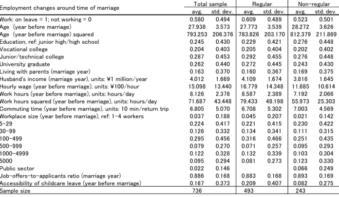
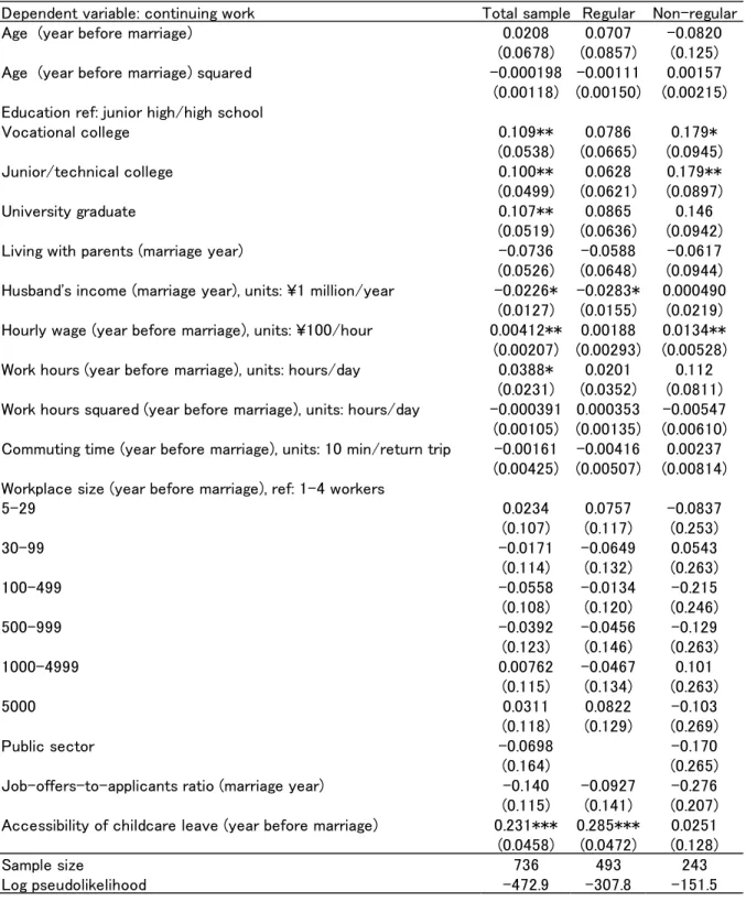
The above-mentioned differences are readily apparent, but we also conducted probit analysis to confirm differences in employment separation rates, controlling for other factors. Table 4 shows descriptive statistics for the sample used for the marriage decision estimation. Table 5 shows the results of probit analysis using the data in Table 4. The data used in the sample is restricted to women who were working the year before marriage. For the dependent variable, women who continued working the year before marriage were assigned a value of 1, and those who quit or changed jobs were assigned a value of 0. The explanatory variables included basic attributes such as age and education as well as a variety of data related to the women’s workplaces in the previous year.
Table 5 shows the following. First, looking at basic attributes, in contrast to the marriage decision estimates, neither age nor age squared provides significant results. Next, the education effect shows that for non-regular employees, the higher the education, the greater the probability of continuing to work. Compared with junior high and high school graduates, women who graduated from technical high schools and junior and technical colleges had employment rates of roughly 17.9 pp higher. As mentioned above, the cost of income foregone and an environment that facilitates continued employment at the original workplace are likely factors. Further, looking at living with parents, in all cases the marginal effect is negative, but not significant, showing that it has no impact on continued employment after marriage.
Further, among work-related influences, commuting time is not significant. In contrast to the decision on marriage, there are no significant differences in women’s continued employment based on the length of commuting time. Hourly wages have a positive and significant impact (+0.41% for every ¥100 in the total case), indicating that higher wages encourage continued employment.
Husband’s income has a negative, significant impact for the total sample and for women in regular employment; it decreases the wife’s employment continuity rates (-2.26% and -2.83% for every ¥100). This accords with one version of the Douglas-Arisawa Law, which has been recognized since 2002. The dummy for number of employees does not show any significant results for any of the variables. The job-offers-to-applicants ratio, a proxy for labor demand, does not yield any significant results. Conversely, looking at work hours, the significant cases had a positive sign; women who worked long hours one year before marriage continued to work
Employed two years before marriage Total Junior high/high school Junior/technical college graduate Bachelor's/Master's degree Urban Regional One year before marriage 0.944 0.943 0.949 0.950 0.937 0.949 Year of marriage 0.763 0.671 0.778 0.812 0.699 0.805 One year after marriage 0.796 0.729 0.801 0.832 0.741 0.833 Two years after marriage 0.827 0.743 0.835 0.871 0.790 0.851 Three years after marriage 0.782 0.686 0.784 0.851 0.748 0.805
Sample size 358 70 176 101 143 215
after marriage (+3.88% per hour). Finally, the availability of childcare leave had a significant, positive impact for the total sample and regular employees (+23.1% to +28.5%). The availability of childcare leave promoted continued female employment around the time of marriage. It is conceivable that whether measures for work-life balance are in place affects whether women continue to work as they may anticipate major life events such as childbirth after marriage. Further, we examined the impact of birth cohorts. For estimation results from the Japanese Panel Survey of Consumers with the sample restricted to regular employees, the dummy for those born in the 1970s and 1980s yielded positive and significant results (compared to those born in the 1960s). Holding other independent variables constant, the decision to continue working after marriage is more likely for the younger generations, but among non-regular workers, the dummy for those born in the 1980s is negative and significant, so the younger generations tend not to continue working. Depending on whether or not the woman has regular employment status before marriage, there is a tendency for an increasing impact on employment continuity after marriage (omitted in the table).
Table 4. Descriptive statistics for the sample used in estimating employment decisions around the time of marriage
Source: Ministry of Health, Labour and Welfare, Longitudinal Survey of Adults in the 21st Century
avg. std. dev. avg. std. dev. avg. std. dev.
Work: on leave = 1; not working = 0 0.580 0.494 0.609 0.489 0.523 0.501
Age (year before marriage) 27.938 3.573 27.773 3.539 28.272 3.626
Age (year before marriage) squared 793.253 206.376 783.826 203.170 812.379 211.869
Education, ref: junior high/high school 0.245 0.430 0.229 0.421 0.276 0.448
Vocational college 0.204 0.403 0.205 0.404 0.202 0.402
Junior/technical college 0.287 0.453 0.292 0.455 0.276 0.448
University graduate 0.262 0.440 0.272 0.445 0.243 0.430
Living with parents (marriage year) 0.163 0.370 0.160 0.367 0.169 0.375
Husband's income (marriage year), units: ¥1 million/year 4.012 1.669 4.109 1.674 3.816 1.645 Hourly wage (year before marriage), units: ¥100/hour 15.098 13.440 16.779 14.348 11.685 10.614 Work hours (year before marriage), units: hours/day 8.126 2.378 8.587 2.389 7.192 2.066 Work hours squared (year before marriage), units: hours/day 71.687 43.448 79.433 48.198 55.973 25.303 Commuting time (year before marriage), units: 10 min/return trip 6.805 5.070 6.708 5.302 7.003 4.569 Workplace size (year before marriage), ref: 1-4 workers 0.037 0.188 0.045 0.207 0.021 0.142
5-29 0.224 0.417 0.221 0.415 0.230 0.422 30-99 0.126 0.332 0.134 0.341 0.111 0.315 100-499 0.295 0.456 0.316 0.466 0.251 0.435 500-999 0.079 0.270 0.071 0.257 0.095 0.293 1000-4999 0.122 0.328 0.132 0.339 0.103 0.304 5000 0.095 0.294 0.081 0.273 0.123 0.330 Public sector 0.022 0.146 0.066 0.249
Job-offers-to-applicants ratio (marriage year) 0.886 0.168 0.883 0.168 0.893 0.169 Accessibility of childcare leave (year before marriage) 0.167 0.373 0.209 0.407 0.082 0.275
Sample size 736 493 243
Employment changes around time of marriage Total sample Regular Non-regular
Table 5. Estimation results: employment decisions around time of marriage (marginal effects)
Source: Ministry of Health, Labour and Welfare, Longitudinal Survey of Adults in the 21st Century Note: The upper rows are marginal effects, and lower rows in parentheses are standard errors. ***significant at the 1% level; ** significant at the 5% level; *significant at the 10% level.
Dependent variable: continuing work Total sample Regular Non-regular
Age (year before marriage) 0.0208 0.0707 -0.0820
(0.0678) (0.0857) (0.125)
Age (year before marriage) squared -0.000198 -0.00111 0.00157
(0.00118) (0.00150) (0.00215) Education ref: junior high/high school
Vocational college 0.109** 0.0786 0.179* (0.0538) (0.0665) (0.0945) Junior/technical college 0.100** 0.0628 0.179** (0.0499) (0.0621) (0.0897) University graduate 0.107** 0.0865 0.146 (0.0519) (0.0636) (0.0942)
Living with parents (marriage year) -0.0736 -0.0588 -0.0617
(0.0526) (0.0648) (0.0944) Husband's income (marriage year), units: ¥1 million/year -0.0226* -0.0283* 0.000490
(0.0127) (0.0155) (0.0219) Hourly wage (year before marriage), units: ¥100/hour 0.00412** 0.00188 0.0134**
(0.00207) (0.00293) (0.00528) Work hours (year before marriage), units: hours/day 0.0388* 0.0201 0.112
(0.0231) (0.0352) (0.0811) Work hours squared (year before marriage), units: hours/day -0.000391 0.000353 -0.00547
(0.00105) (0.00135) (0.00610) Commuting time (year before marriage), units: 10 min/return trip -0.00161 -0.00416 0.00237
(0.00425) (0.00507) (0.00814) Workplace size (year before marriage), ref: 1-4 workers
5-29 0.0234 0.0757 -0.0837 (0.107) (0.117) (0.253) 30-99 -0.0171 -0.0649 0.0543 (0.114) (0.132) (0.263) 100-499 -0.0558 -0.0134 -0.215 (0.108) (0.120) (0.246) 500-999 -0.0392 -0.0456 -0.129 (0.123) (0.146) (0.263) 1000-4999 0.00762 -0.0467 0.101 (0.115) (0.134) (0.263) 5000 0.0311 0.0822 -0.103 (0.118) (0.129) (0.269) Public sector -0.0698 -0.170 (0.164) (0.265)
Job-offers-to-applicants ratio (marriage year) -0.140 -0.0927 -0.276 (0.115) (0.141) (0.207) Accessibility of childcare leave (year before marriage) 0.231*** 0.285*** 0.0251 (0.0458) (0.0472) (0.128)
Sample size 736 493 243
Log pseudolikelihood -472.9 -307.8 -151.5
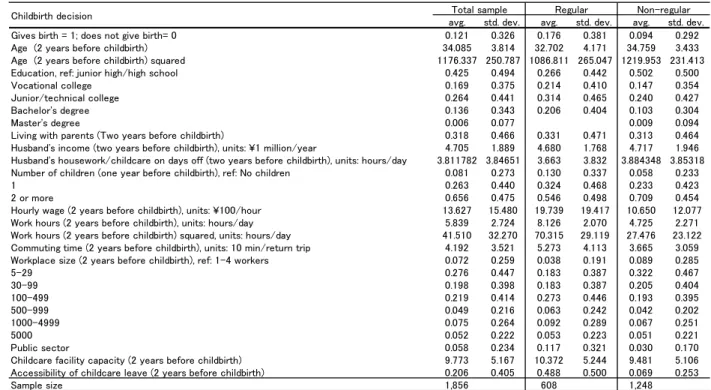
6. Childbirth decisions
In this section, we use the Longitudinal Survey of Adults in the 21st Century to examine what factors affect the decision on whether to have children. Table 6 shows descriptive statistics for the sample used in the childbearing decision estimation. We conducted probit analysis, with the dependent variable taking a value of 1 for women who gave birth and 0 for those who did not. As before, the explanatory variables used were basic characteristics of the women themselves and information regarding their place of employment. We also used childcare facility capacity by prefecture and information about the husband’s income and hours spent on housework and childcare. Further, to take into account pre-pregnancy factors, given that the normal gestational period spans roughly 40 weeks, we used data from two years before childbirth rather than the year before.
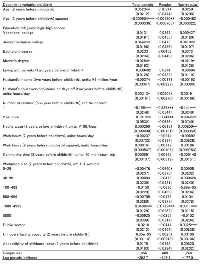
Table 7 shows estimation results from which we draw the following conclusions. First, age and age squared show positive and negative signs, respectively (+5.23%, -0.10% in the total sample case), and are significant in the total sample and regular employees cases. As a result, the age effect means that the number of women giving birth increases, but the number of women giving birth declines after a peak age.
The education dummy is not significant in most cases, but where it is significant, the likelihood of giving birth is relatively high for graduates of junior and technical colleges (+4.42%) compared with junior high and high school graduates. Conversely, the sign for women with a master’s degree is negative, suggesting relatively lower fertility (-2.84%)4. We expected a positive result for living with parents because it means there are household resources available to help with childcare, but there were no significant results.
Next, we turn to information regarding women’s employment. In no case was there was any significant impact from commuting time. Regarding hourly wages, in the non-regular employment case, the effect was positive and significant (+0.08% for every ¥100), encouraging the decision to have a child among women in non-regular employment before childbirth. There were no significant results for the husband’s income. In many cases workplace size was not significant, but in the significant cases the sign was always negative. Compared to a small (1-4 employee) workplace, the bigger the company where a woman works, the lower the likelihood of giving birth.
Looking at number of children, women who already had one child, and those who had at least two children, at one year before childbirth were less likely to give birth than those with no children (-19.5% and -78.1%, respectively). There were no significant results for childcare facility capacity. For work hours and work hours squared, there were no significant results in all cases. The availability of childcare leave had positive effects, though not significant. For husband’s hours spent on housework and childcare on days off in the total sample case and the
4 In the regular employment case, the sample with a master’s degree does not exist. This sample is very few; only 0.6% has a master’s degree in the total sample.
17
regular employee case, the result was positive and significant. The longer the husband spent on housework and childcare on his days off, the more likely the woman was to give birth (+0.31%, +0.51%).
Next, we used the Japanese Panel Survey of Consumers to examine the impact of birth cohort. The dummy for those born in the 1970s was positive and significant (compared to those born in the 1960s), suggesting that the likelihood of choosing to have children rises with birth cohort (not shown in the table). It is necessary to consider that there may be an issue with the sample itself. We analyzed the sample controlling for women aged 26-34 years, but the age of mothers giving birth is rising, and in recent years, the number of women in this age bracket giving birth is increasing, and it is possible that this is making it appear that the birth rate is increasing. Rather than more women in the 1970s birth cohort choosing to have children than the 1960s birth cohort, it may be the case that the likelihood of choosing to have children is rising for rich information on their late 20s and early 30s in the 1970s birth cohort, the age of the respondents (26-34 years)5 in the Japanese Panel Survey of Consumers sample used for estimations. Regarding this point, it will be necessary in the future to refine the analysis using historical data.
Table 6. Descriptive statistics for the sample used in the childbirth decision estimation
Source: Ministry of Health, Labour and Welfare, Longitudinal Survey of Adults in the 21st Century
5 In estimates with a dummy for birth cohort added, the age distribution for each cohort was taken into account, and restricted to respondents aged 25-34 years for all cohorts.
avg. std. dev. avg. std. dev. avg. std. dev.
Gives birth = 1; does not give birth= 0 0.121 0.326 0.176 0.381 0.094 0.292
Age (2 years before childbirth) 34.085 3.814 32.702 4.171 34.759 3.433
Age (2 years before childbirth) squared 1176.337 250.787 1086.811 265.047 1219.953 231.413
Education, ref: junior high/high school 0.425 0.494 0.266 0.442 0.502 0.500
Vocational college 0.169 0.375 0.214 0.410 0.147 0.354
Junior/technical college 0.264 0.441 0.314 0.465 0.240 0.427
Bachelor's degree 0.136 0.343 0.206 0.404 0.103 0.304
Master's degree 0.006 0.077 0.009 0.094
Living with parents (Two years before childbirth) 0.318 0.466 0.331 0.471 0.313 0.464
Husband's income (two years before childbirth), units: ¥1 million/year 4.705 1.889 4.680 1.768 4.717 1.946 Husband's housework/childcare on days off (two years before childbirth), units: hours/day 3.811782 3.84651 3.663 3.832 3.884348 3.85318 Number of children (one year before childbirth), ref: No children 0.081 0.273 0.130 0.337 0.058 0.233
1 0.263 0.440 0.324 0.468 0.233 0.423
2 or more 0.656 0.475 0.546 0.498 0.709 0.454
Hourly wage (2 years before childbirth), units: ¥100/hour 13.627 15.480 19.739 19.417 10.650 12.077
Work hours (2 years before childbirth), units: hours/day 5.839 2.724 8.126 2.070 4.725 2.271
Work hours (2 years before childbirth) squared, units: hours/day 41.510 32.270 70.315 29.119 27.476 23.122 Commuting time (2 years before childbirth), units: 10 min/return trip 4.192 3.521 5.273 4.113 3.665 3.059
Workplace size (2 years before childbirth), ref: 1-4 workers 0.072 0.259 0.038 0.191 0.089 0.285
5-29 0.276 0.447 0.183 0.387 0.322 0.467 30-99 0.198 0.398 0.183 0.387 0.205 0.404 100-499 0.219 0.414 0.273 0.446 0.193 0.395 500-999 0.049 0.216 0.063 0.242 0.042 0.202 1000-4999 0.075 0.264 0.092 0.289 0.067 0.251 5000 0.052 0.222 0.053 0.223 0.051 0.221 Public sector 0.058 0.234 0.117 0.321 0.030 0.170
Childcare facility capacity (2 years before childbirth) 9.773 5.167 10.372 5.244 9.481 5.106
Accessibility of childcare leave (2 years before childbirth) 0.206 0.405 0.488 0.500 0.069 0.253
Sample size 1,856 608 1,248
Childbirth decision Total sample Regular Non-regular
18
Table 7. Results (marginal effects) for the childbirth decision estimation
Note: The upper rows are marginal effects, and lower rows in parentheses are standard errors. ***significant at the 1% level; ** significant at the 5% level; *significant at the 10% level. 7. Changes in employment after childbirth
Dependent variable: childbirth Total sample Regular Non-regular Age (2 years before childbirth) 0.0523** 0.105** 0.0250
(0.0212) (0.0474) (0.0208) Age (2 years before childbirth) squared -0.000904*** -0.00180** -0.000462
(0.000336) (0.000763) (0.000322) Education ref: junior high/high school
Vocational college 0.0131 0.0387 0.000427 (0.0191) (0.0455) (0.0180) Junior/technical college 0.0442** 0.0473 0.0419** (0.0196) (0.0436) (0.0197) Bachelor's degree 0.0233 0.00453 0.0372 (0.0234) (0.0449) (0.0286) Master's degree -0.0284* -0.0219* (0.0162) (0.0126) Living with parents (Two years before childbirth) -0.000492 0.0274 -0.00694 (0.0128) (0.0332) (0.0119) Husband's income (two years before childbirth), units: ¥1 million/year -0.00374 -0.00148 -0.00192 (0.00347) (0.00927) (0.00300) Husband's housework/childcare on days off (two years before childbirth),
units: hours/day 0.00313* 0.00505* 0.00191 (0.00161) (0.00270) (0.00166) Number of children (one year before childbirth), ref: No children
1 -0.195*** -0.325*** -0.141***
(0.0248) (0.0544) (0.0240) 2 or more -0.781*** -0.774*** -0.804***
(0.0532) (0.0636) (0.0740) Hourly wage (2 years before childbirth), units: ¥100/hour 0.000290 -0.00131 0.000850**
(0.000400) (0.00161) (0.000359) Work hours (2 years before childbirth), units: hours/day -0.00237 -0.0244 -0.00692
(0.00733) (0.0187) (0.00826) Work hours (2 years before childbirth) squared, units: hours/day 0.000161 0.00112 0.00106
(0.000547) (0.00106) (0.000753) Commuting time (2 years before childbirth), units: 10 min/return trip 0.000591 0.00192 -0.000140 (0.00137) (0.00319) (0.00151) Workplace size (2 years before childbirth), ref: 1-4 workers
5-29 -0.00476 -0.0640* 0.00905 (0.0237) (0.0373) (0.0232) 30-99 -0.00883 -0.0479 -0.000426 (0.0239) (0.0431) (0.0240) 100-499 -0.0150 -0.0630 -5.68e-05 (0.0220) (0.0469) (0.0234) 500-999 -0.00705 -0.0475 0.0104 (0.0280) (0.0377) (0.0378) 1000-4999 -0.0408*** -0.0729*** -0.0311*** (0.0129) (0.0252) (0.0115) 5000 -0.00925 -0.0356 -0.0102 (0.0308) (0.0547) (0.0234) Public sector -0.0218 -0.0444 -0.0325*** (0.0212) (0.0454) (0.00838) Childcare facility capacity (2 years before childbirth) -6.05e-05 -0.00254 0.00100
(0.00114) (0.00248) (0.00106) Accessibility of childcare leave (2 years before childbirth) 0.0175 0.0465 0.00820
(0.0163) (0.0294) (0.0232)
Sample size 1,856 608 1,248
Log pseudolikelihood -292.7 -105.1 -177.0
In this section, we use the Longitudinal Survey of Adults in the 21st Century to examine employment rates after childbirth. Table 8 shows data for women who were working two years before childbirth, regardless of birth order. It shows the percentage of women who were working one year before childbirth, in the childbirth year, and one, two and three years after childbirth, by education and whether they lived in urban or regional areas. Employment rates are roughly 75% in the year before childbirth and drop sharply to roughly 50% in the childbirth year. However, from one year after childbirth onward they turn upward, climbing to 63%, but even three years after childbirth, employment levels have not returned to those that prevailed one year before childbirth.
The data confirm that the decline in employment rates from one year before childbirth to the childbirth year is lower for highly educated women (roughly 55% at childbirth) than junior high or high school graduates (around 41% at childbirth). Conversely, the increase in employment rates from the childbirth year to one year after childbirth is larger for junior high or high school graduates. Similar to changes in employment after marriage, the gap due to education gradually shrinks over time. Looking at the urban/regional split, employment rates one year before childbirth and during the childbirth year are higher for urban areas, but from one year after childbirth, employment rates in regional areas overtake those in the urban areas. This accords with previous research (Unayama, 2011), which noted differences in employment separation rates by prefecture at the time of marriage or childbirth.
Tables 9 and 10 show employment rates over time following the birth of the first child or a second or subsequent child. The drop in employment rates from one year before childbirth to the childbirth year is more pronounced in the case of the first child. In these instances, employment rates in the childbirth year are around half the levels of the year before. For the second and subsequent children, employment rates in the childbirth year are around four-fifths of the level the year before childbirth.
Table 8. Employment rates before/after childbirth by education and location
Source: Ministry of Health, Labour and Welfare, Longitudinal Survey of Adults in the 21st Century
Note: “Urban” = Tokyo, Saitama, Chiba, Kanagawa, Hyogo, Osaka, Kyoto. “Regional” is all other prefectures. The sample covers only those respondents who answered in all years.
Employed two years before childbirth Total Junior high/high school Junior/technical college Bachelor's/Master's degree Urban Regional Year before childbirth 0.755 0.733 0.765 0.751 0.778 0.745 Childbirth year 0.505 0.412 0.545 0.541 0.518 0.500 1 year after childbirth 0.554 0.508 0.570 0.580 0.545 0.558 2 years after childbirth 0.590 0.562 0.602 0.601 0.568 0.600 3 years after childbirth 0.631 0.611 0.648 0.609 0.593 0.647
Sample size 1326 386 596 281 396 930
Table 9. Employment rates after birth of the first child
Source: Ministry of Health, Labour and Welfare, Longitudinal Survey of Adults in the 21st Century
Note: “Urban” indicates Tokyo, Saitama, Chiba, Kanagawa, Hyogo, Osaka, and Kyoto. “Regional” indicates all other prefectures.
Sample covers only those respondents who answered in all years. Table 10. Employment rates after birth of a second or subsequent child
Source: Ministry of Health, Labour and Welfare, Longitudinal Survey of Adults in the 21st Century
Note: “Urban” indicates Tokyo, Saitama, Chiba, Kanagawa, Hyogo, Osaka, and Kyoto. “Regional” indicates all other prefectures.
The sample covers only those respondents who answered in all years.
Next, we examine which factors affect the employment status of women one year after childbirth among those who were working one year before giving birth. Table 11 shows descriptive statistics for the sample used in the following employment decision estimation. Table 12 shows the results of probit analysis of the data sample in Table 11. We restricted the sample to women who were working the year before they gave birth, and the dependent variable takes a value of 1 for women who continued working and 0 for those who did not continue working. In addition to the women’s basic attributes, we used various data concerning their work, spouses, and families as independent variables in our estimations.
We draw the following conclusions from Table 12. First, looking at the women’s basic attributes, education do not give significant results regarding their effect on the decision to work after giving birth to the same extent as choosing marriage or childbirth or choosing to work after marriage. Continued employment was significantly higher than among regular employees who graduated from vocational school compared with junior high or highs school. Notably, commuting time to the company they worked at had a big impact. For the entire sample and women in the regular employment, commuting time had a significant and negative impact (-1.3% to -1.9% for every 10 min). It was not significant for the non-regular employees, but the sign was also negative. From this, it is apparent that in many cases women who had a long commute to work took childbirth as an opportunity to quit work. Conversely, the results for
Employed two years before childbirth Total Junior high/high school Junior/technical college Bachelor's/Master's degree Urban Regional Year before childbirth 0.716 0.717 0.718 0.706 0.748 0.700 Childbirth year 0.393 0.277 0.422 0.447 0.412 0.384 1 year after childbirth 0.433 0.326 0.460 0.482 0.460 0.419 2 years after childbirth 0.464 0.386 0.486 0.503 0.472 0.460 3 years after childbirth 0.503 0.440 0.529 0.518 0.508 0.501
Sample size 763 184 348 197 250 513
Employed two years before childbirth Total Junior high/high high school Junior/technical college Bachelor's/Master's degree Urban Regional Year before childbirth 0.808 0.748 0.831 0.857 0.829 0.801 Childbirth year 0.657 0.535 0.718 0.762 0.699 0.643 1 year after childbirth 0.719 0.673 0.726 0.810 0.692 0.729 2 years after childbirth 0.762 0.723 0.766 0.833 0.733 0.772 3 years after childbirth 0.805 0.767 0.815 0.821 0.740 0.827
Sample size 563 202 248 84 146 417
hourly wage rates are positive and significant, suggesting that higher rates encourage continued employment (+0.92% to +1.24% for every ¥100).
Looking at results for work hours and work hours squared, there are positive and negative effects, respectively, for the total sample and for women in regular employment. Women who were working long hours one year before giving birth were more likely to continue working one year after giving birth (+10.2% to +20.1%), but as working hours increase, the likelihood of continuing to work tapers off. In all cases the accessibility of childcare leave had a significant, positive effect (+28.6% to +35.6%), so it encourages women to keep working.
We next look at family effects. The impact of the husband’s income is negative and significant, discouraging continued employment by the wife (-3.07% to -4.63% per ¥1 million). The impact of the husband’s income decile on reducing the wife’s employment rates appears to be waning over the long term (Ministry of Health, Labour and Welfare, 2014), but our results confirm that the husband’s income is still a factor in the wife’s decision on whether to continue employment at the time of marriage or childbirth. Turning to living with the parents, the marginal effect is positive, as was the case with the decision to work after marriage, but there were no significant results.
We now turn to estimation results using a dummy variable for the birth order of the child. It is found that women who give birth to a second or third child are more likely to continue working than those who give birth to their first child. This indicates a strong tendency to continue working after having a second or third child among women who continue working after having their first child. The job-offers-to-applicants ratio in the childbirth year, a proxy variable for labor market demand, has a positive sign, but there are no significant results. Turning to childcare facility capacity, we see that the higher it is, the higher the likelihood that the mother will continue to work one year after giving birth for the total sample (+0.99%). This is in line with results from previous research showing that the provision of childcare facilities has an effect of women continuing employment (Shigeno and Okusa, 1999; Higuchi et al., 2007; Unayama, 2011). Finally, using the Japanese Panel Survey of Consumers to gauge the impact of birth cohort, with other independent variables held constant, there are differences between regular and non-regular employees in the sign of the marginal effect from the birth cohort dummy: It is positive for the former and negative for the latter. In particular, for non-regular workers born in the 1980s, there is a declining tendency to remain in employment after giving birth (not shown in the table).
Table 11. Descriptive statistics for the sample used in the employment decision estimation for around the time of childbirth
Source: Ministry of Health, Labour and Welfare, Longitudinal Survey of Adults in the 21st Century
avg. std. dev. avg. std. dev. avg. std. dev. Work: on leave = 1; not working = 0 0.597 0.491 0.681 0.467 0.478 0.501 Age (year before childbirth) 29.568 3.426 29.056 3.511 30.294 3.172 Age (year before childbirth) squared 885.989 202.223 856.523 205.400 927.733 190.399 Education, ref: junior high/high school 0.332 0.471 0.307 0.462 0.368 0.483 Vocational college 0.225 0.418 0.245 0.431 0.197 0.399 Junior/technical college 0.245 0.430 0.241 0.429 0.250 0.434 Bachelor's degree 0.183 0.387 0.198 0.399 0.162 0.370 Master's degree 0.015 0.120 0.009 0.096 0.022 0.147 Living with parents (childbirth year) 0.261 0.440 0.272 0.446 0.246 0.431 Husband's income (childbirth year), units: ¥1 million/year 4.225 1.986 4.051 1.779 4.471 2.227 Birth order of child; ref: first child 0.530 0.500 0.570 0.496 0.474 0.500 Second 0.194 0.396 0.192 0.394 0.197 0.399 Third or subsequent 0.276 0.447 0.238 0.427 0.329 0.471 Hourly wage (year before childbirth), units: ¥100/hour 15.281 16.636 18.262 17.503 11.059 14.334 Work hours (year before childbirth), units: hours/day 7.059 2.625 8.139 2.121 5.528 2.509 Work hours (year before childbirth) squared, units: hours/day 56.704 33.655 70.735 30.470 36.828 27.392 Commuting time (year before childbirth), units: 10 min/return trip 5.735 5.418 6.037 4.744 5.308 6.235 Workplace size (year before childbirth), ref: 1-4 workers 0.051 0.220 0.040 0.197 0.066 0.248 5-29 0.269 0.444 0.186 0.390 0.386 0.488 30-99 0.142 0.349 0.158 0.365 0.118 0.324 100-499 0.267 0.443 0.319 0.467 0.193 0.396 500-999 0.078 0.268 0.093 0.291 0.057 0.232 1000-4999 0.085 0.280 0.096 0.295 0.070 0.256 5000 0.089 0.285 0.108 0.311 0.061 0.241 Public sector 0.020 0.140 0.048 0.215
Job-offers-to-applicants ratio (childbirth year) 0.886 0.169 0.901 0.158 0.866 0.183 Childcare facility capacity (childbirth year) 10.044 5.196 10.483 5.260 9.421 5.050 Accessibility of childcare leave (year before childbirth) 0.236 0.425 0.337 0.474 0.092 0.290
Sample size 551 323 228
Regular Non-regular Changes in employment around childbirth Total sample