大阪府立大学　学術情報リポジトリ

(1)

Analog Impairments Compensation in OFDM

Direct-Conversion Receiver

著者

Umut Yunus

内容記述

学位授与大学: Osaka Prefecture University(大阪

府立大学), 学位の種類: 博士(工学), 学位記番号:

論工第1245号, 学位授与年月日: 2010-03-31, 指導

教員: 山下勝己.

(2)

Analog Impairments Compensation in

OFDM Direct-Conversion Receiver

Umut Yunus

February 2010

(3)

(4)

Analog Impairments Compensation in

OFDM Direct-Conversion Receiver

A dissertation submitted to the

Graduate School of Engineering

in partial fulfillment of

the requirements for the

degree of Doctor of Engineering

Umut Yunus

Sakai, February, 2010

INTELLIGENTINFORMATIONCOMMUNICATIONLABORATORY Department of Electrical & Electronic Systems Graduate School of Engineering Osaka Prefecture University

(5)

Copyright ⃝ 2010 Umut Yunusc . Submitted version, January, 2010. Revised version, February, 2010.

Typeset by the author with the LA_{TEX 2}_{ε Documentation System, with AMS-L}A_{TEX Extensions, in 12/18pt} Sabon and Pazo Math fonts.

INTELLIGENTINFORMATIONCOMMUNICATIONLABORATORY Department of Electrical & Electronic Systems

Graduate School of Engineering Osaka Prefecture University

(6)

Acknowledgments

W

ITH utmost sincerity, I would like to express my gratitude to my supervisor, Professor Katsumi Yamashita for his constant encouragement and valuable ad-vices that guided me throughout this research, and for his enthusiasm and devotion that always inspired me during my hard times. My deepest thanks go to Prof. Yamashita.

I would like to thank Professors Yutaka Katsuyama, Masaharu Ohashi, for serving as members of my dissertation committee and their vital suggestions. They assured the quality of this research.

I am specially grateful to Dr. Hai Lin for his encouragement and full support during my hard time. I would like to thank all my colleagues in the Intelligent Information Communication lab, for their great support.

I would also like to gratefully acknowledge the financial support received from the Japanese Government-Monbu Kagakusho Scholarship.

I would like to thank Professors Masanobu Kominami and Yiwei He in Osaka Electro-Communication University for their valuable advices and encouragement.

I would like to thank Xinjiang University for their great support. I am specially grateful to Professors Zhenhong Jia and Dilmurat Tursun for their encouragement and full support.

Finally, I am extremely grateful to my family for all their unconditional support, patience, trust and love during these hard times while I was working at a distance. I dedicate this work to them.

(7)

(8)

List of Figures

2.1 Trends of wireless systems . . . 10

2.2 Multipath channel . . . 11

2.3 Comparison of spectral efficiency . . . 12

2.4 OFDM system model. . . 13

2.5 BER versus SNR . . . 15

2.6 Superheterodyne receiver. . . 18

2.7 Direct-conversion receiver. . . 18

2.8 Spectrum shift of OFDM due to CFO . . . 20

2.9 Model of CFO. . . 21

2.10 Model of I/Q imbalance. . . 23

2.11 Model of DC offset. . . 24

2.12 Spectrum of DC offset. . . 24

3.1 IEEE 802.11a preamble. . . 26

3.2 Mathematical model. . . 27

3.3 Model of the residual TV-DCO. . . 28

3.4 CFO MSE to various f_d, fc =10kHz . . . 35

3.5 TV-DCO MSE versus SNR, fc =10kHz, fd =200Hz . . . 36

3.6 CFO MSE to various fc, fd =200Hz . . . 37

3.7 CFO MSE versusε, f_c =100kHz,f_d =200Hz,SNR=20dB . . . 38

3.8 BER versus SNR, fc =100kHz, fd =200Hz . . . 39

4.1 STS preamble and TV-DCO model. . . 42

4.2 Architecture of a DCR. . . 44

4.3 Mathematical model of the system. . . 44

4.4 CFO MSE versus SNR, fx =100kHz,g =1.25,ϕ=6◦,ε=0.2 . . . . 51

4.5 CFO MSE versusε, f_x =100kHz, g=1.25,ϕ=6◦, SNR=25dB . . . 52

4.6 IRR versus SNR, fx =100kHz,g=1.25,ϕ=6◦, ε=0.2 . . . 53

(13)

viii LIST OF FIGURES

4.7 BER versus SNR, fx =100kHz,g=1.25,ϕ=6◦, ε=0.2 . . . 54

5.1 Decomposition model of channel matrix. . . 61

5.2 Transmitter and receiver diagram. . . 63

5.3 Decomposition model of channel matrix in proposed method. . . 63

5.4 Power of ISI versus sampling time, after FDE. . . 68

5.5 SER versus SNR, QPSK. . . 70

5.6 SER versus SNR, 16QAM. . . 71

(14)

List of Tables

3.1 Computational complexity . . . 32 3.2 Simulation setup . . . 33 4.1 Simulation setup . . . 50

(15)

(16)

List of Acronyms

ADSL Asymmetric Digital Subscriber Line

AGC Automatic Gain Control

AWGN Additive White Gaussian Noise

BER Bit Error Rate

BPSK Binary Phase Shift Keying

CATV Cable Television

CFO Carrier Frequency Offset

CP Cyclic Prefix

DAB Digital Audio Broadcasting

DCR Direct-Conversion Receiver

DCO DC Offset

DFT Discrete Fourier Transform

DMC Differential Method Coarse estimation

DMF Differential Method Fine estimation

DSP Digital Signal Processor

DVB Digital Video Broadcasting

FDE Frequency Domain Equalization

FDM Frequency Division Multiplexing

(17)

xii List of Acronyms

FFT Fast Fourier Transform

FIR Finite Impulse Response

FTTH Fiber To The Home

GI Guard Interval

HPF High Pass Filter

HSDPA High Speed Downlink Packet Access

ICI Inter-Carrier Interference

IDFT Inverse Discrete Fourier Transform

IF Intermediate Frequency

IFFT Inverse Fast Fourier Transform

IICM Iteration based ISI Cancellation Method

I/Q In phase / Quadrature phase

IRR Image Rejection Ratio

ISI Inter-Symbol Interference

ISM Industrial, Scientific and Medical

LMC Least square Method Coarse estimation

LMF Least square Method Fine estimation

LNA Low Noise Amplifier

LO Local Oscillator

LPF Low Pass Filter

LTS Long Training Sequence

MC-CDMA Multi-Carrier Code Division Multiple Access

(18)

xiii

MUI Multi-User Interference

OFCDM Orthogonal Frequency and Code Division Multiplexing

OFDM Orthogonal Frequency Division Multiplexing

PICM Proposed ISI Cancellation Method

PP Periodic Pilot

P/S Parallel to Serial

QAM Quadrature Amplitude Modulation

QPSK Quadrature Phase Shift Keying

RF Radio Frequency

SER Symbol Error Rate

S/P Serial to Parallel

STS Short Training Sequence

SNR Signal to Noise Ratio

TV-DCO Time-Varying DCO

VSF Variable Spreading Factor

(19)

(20)

C H A P T E R

1

Introduction

T

HE history of wireless communications began in 1886, when Hertz generated elec-tromagnetic waves. Around 1897, Marconi successfully demonstrated wireless telegraphy, for that he was awarded the Nobel Price in 1909. Based on this, the radio communication by Morse code across the Atlantic Ocean had been established in 1901. More than one century has passed, since then. Today, telecommunication has become so indispensable that we almost cannot imagine our lives without it. From satellite transmis-sion, radio and television broadcasting to the now ubiquitous mobile telephone, wireless communications have revolutionized human society. In contrast to the poor information-carrying ability of the early telecommunication system, instantaneous transferring of a large number of information, such as multimedia information, becomes possible.

Under the increasing demand to high-speed, high-spectral efficiency of radio com-munication, the digital-communication employing orthogonal frequency division mul-tiplexing (OFDM) had emerged. The origin of OFDM started in 1966, when Chang proposed the structure of OFDM in [32], where the concept of using orthogonal overlap-ping multi-tone signals was given. At that time, although the theory of OFDM was well developed, the implementation of OFDM systems still had some difficulties [33, 34] due to the hardware. In 1971, Weinstein [34] introduced the idea of using a discrete Fourier transform (DFT) to perform baseband modulation and demodulation of the signals.This presented an opportunity of an easy implementation of OFDM, especially with the use of fast Fourier transform (FFT). Another important contribution was due to Peled and Ruiz in 1980 [3], who introduced the cyclic prefix (CP) to combat mutipath fading. Then, communication of OFDM had become possible according to the development of digital

(21)

2 Introduction

signal processor (DSP) circuit. As a result, in 1987, OFDM was used in the European digital audio broadcasting (DAB) standard. Nowadays, OFDM is well-known modula-tion scheme, which has been adopted in many wireless communicamodula-tion systems such as DAB, digital video broadcasting (DVB), and IEEE 802.11 wireless local area network (WLAN) [1].

1.1 T

ENDENCY OF

W

IRELESS

C

OMMUNICATION

S

YSTEMS

The total number of mobile subscribers is about 100 million in Japan, which increased 10 times in 10 years. At the end of 2005, there were 80 million internet subscribers in Japan, that occupied 62% of the population [20]. There were 20 million broadband users,

accessing from asymmetric digital subscriber line (ADSL), fiber to the home (FTTH), and cable television (CATV) [20]. In 2005, the number of 3G subscribers is 41 million [20].

As a 3.5G system, high speed downlink packet access (HSDPA) was used to start the service in 2006, and can achieve a transmission speed of up to 14 Mbit/s, even when using the same 5MHz frequency bandwidth as 3G [20]. As a 3.9G system, transmission speed of 100 Mbit/s can be achieved at the downlink [17]. This means that the trans-mission speed of cellular phone increased 10 thousand times during these 20 years. As a result, the cellular phone, which was just used for audio communication, is able to ac-cess multimedia freely. For next generation systems, a very high-speed wireless acac-cess of approximately 1 Gbit/s is required. One possible technology that satisfies the require-ments is variable spreading factor orthogonal frequency and code division multiplexing (VSF-OFCDM) .

On the other hand, IEEE 802.11g, which uses OFDM technology in the 2.4 GHz band with a bit rate of 54 Mbit/s, was established in 2003 [20]. Currently, a new standard, IEEE 802.11n can achieve maximum 600 Mbit/s. Furthermore, new standards IEEE 802.11ac and IEEE 802.11ad, which are expected beyond 1Gbit/s in the future, have being discussed [17].

1.2 T

HE

R

ECEIVER

A

RCHITECTURE

According to the receiver architecture, the receivers can be classified to the superhetero-dyne receiver and direct-conversion receiver (DCR). In the following subsection, we will

(22)

1.3 A Brief Review of OFDM-DCR 3

give brief explanations to these receivers.

1.2.1 Superheterodyne Receiver

The superheterodyne principle was introduced in 1918 by the U.S. Army major Edwin Armstrong in France during World War I, which is generally thought to be the receiver of choice owing to its high selectivity and sensitivity. About 98% of radio receivers use this architecture. In a superheterodyne receiver, the input signal is first converted by an offset-frequency local oscillator to a lower intermediate frequency (IF), and substantially amplified in a tuned IF containing highly-selective passive bandpass filters. Therefore, the superheterodyne receiver needs two stages of detection and filtering.

1.2.2 Direct-Conversion Receiver

Direct-conversion receiver (DCR) is very attractive by its smaller size, lower cost, and lower power consumption over the traditional superheterodyne receivers. DCR, also known as homodyne, synchrodyne, or zero-IF receiver was developed in 1932 by a team of British scientists searching for a method to surpass the superheterodyne. DCR is a radio receiver that demodulates the incoming signal by a local oscillator signal synchro-nized in frequency to the carrier of the wanted signal. Therefore, the wanted modulation signal is obtained immediately by low-pass filtering, without further detection. Thus a direct-conversion receiver requires only a single stage of detection and filtering.

1.3 A B

RIEF

R

EVIEW OF

OFDM-DCR

In recent years, OFDM-DCR system, which is a combination of OFDM technique with DCR, has attracted a lot of attention. The main reason is that, in OFDM-DCR, not only high-speed and high spectral efficiency, but also small size, low cost, and low power consumption can be achieved. Although OFDM-DCR has many considerable merits, it leads to additional analog impairments, which causes severe performance degradation of the system. In OFDM-DCR, carrier frequency offset (CFO), DC offset (DCO), and I/Q (in-phase and quadrature-phase) imbalance [4] are considered to be the most serious impairments. In order to obtain good performance, it is necessary to estimate and com-pensate the analog impairments. In this thesis, we focus on the compensation of these analog impairments. To better understand the background of this study, we will give brief reviews of above mentioned analog impairments.

(23)

4 Introduction

1.3.1 CFO

The main drawback of OFDM systems is it’s sensitivity to carrier frequency offset (CFO). Orthogonality among subcarriers is the fundamental of OFDM systems. CFO, mainly caused by frequency mismatch between the transmitter and receiver local oscil-lators (LOs). While CFO occurs, the spectrum of the received signal will be shifted. This will destroy the required orthogonality and result in severe performance degrada-tion. Therefore, the estimation/compensation of CFO is very crucial in OFDM systems. Conventionally, the CFO can be estimated easily from the autocorrelation of periodic pilot (PP) [14, 26, 30, 40].

1.3.2 DCO and I/Q Imbalance

DCO is induced by the self-mixing associated with the imperfect isolation and is known as the most serious problem [2] of DCR. The I/Q imbalance is caused by the mismatched components between the in-phase (I) and quadrature-phase (Q) branches, i.e., is basi-cally any mismatch between the I and Q branches from the ideal case. Therefore, the estimation/compensation of CFO in the presence of I/Q imbalance and the DCO is a critical problem in an OFDM-DCR.

In the absence of DCO, the CFO can be estimated easily from the autocorrelation of periodic pilot (PP) [14, 26, 30, 40]. The CFO estimators in the presence of DCO and of I/Q imbalance in OFDM DCRs have been proposed in [7,12,15,37] and [9,11,19,35,36], respectively. Also, the joint estimation of CFO, I/Q imbalance and DCO can be found in [12]. However, all of these works treated the DCO as time-invariant.

1.3.3 Time-Varying DCO Caused by AGC

In practice, automatic gain control (AGC) is usually used to keep the received signal amplitude proper fixed level. Also, a high pass filter (HPF) is often employed in the DCR to reduce DCO [47]. Therefore, the gain shift in the low noise amplifier (LNA) will cause a time-varying DCO (TV-DCO) [38], whose high frequency components may pass through the HPF. As a result, the ordinary CFO estimation in [7, 12, 15, 37] will be corrupted by the residual TV-DCO. Until now, there is only one CFO estimator tak-ing the residual TV-DCO into account [25]. In this scheme, a differential filter is used to eliminate the residual TV-DCO, and then the CFO is estimated by the conventional autocorrelation-based method. Since the differential filter increases the noise variance and the residual TV-DCO cannot be eliminated completely, this method will cause

(24)

per-1.4 Inter-Symbol Interference Cancellation in OFDM Systems without Guard

Interval 5

formance loss. To the best of our knowledge, until now, only [24] considered the scenario of the coexistence of CFO, I/Q imbalance, and TV-DCO. The idea in [24] is to employ a differential filter to ease the effect of the TV-DCO, and then estimate the CFO by the conventional autocorrelation-based method. However, the differential filter not only fails to completely eliminate the TV-DCO, but also enhances the noise. Also, the CFO es-timation is severely biased by the remaining uncompensated I/Q imbalance. Moreover, in [24], only a CFO estimator was proposed and how to estimate/compensate the I/Q imbalance in this situation was not mentioned.

1.4 I

NTER

-S

YMBOL

I

NTERFERENCE

C

ANCELLATION

IN

OFDM S

YSTEMS WITHOUT

G

UARD

I

NTERVAL

The one reason of that OFDM has been selected for high-speed communication systems, is its good performance in multipath channels. In order to fight multipath, the cyclic prefix (CP), which is also referred to as guard interval (GI), is inserted between symbols. While the length of GI is longer than channel delay spread, it can protect received signal from inter-symbol interference (ISI). However, the price is the transmission speed.

On the other hand, in order to increase the transmission speed, several attempts [8, 13, 18, 21–23, 31, 39, 48] have been made to the cancellation of ISI and ICI (inter-carrier interference) in the OFDM systems with insufficient GI [8, 13, 18, 21–23, 31] or without GI [39, 48]. In [21, 31], time domain equalizer is used to shorten the channel impulse response to combat ISI and ICI. FIR (Finite impulse response) tail cancellation and FIR cyclic reconstruction techniques are used in [18] to cope with ISI and ICI. Pre-coding techniques and oversampling techniques are used to mitigate ISI and ICI in [22] and [23], respectively. In [8, 13], a decision feed back loop is proposed, which not only result in feedback delay increment and error propagation, but also increase the computa-tional complexity. All these methods only consider the OFDM systems with insufficient GI. Since GI insertion reduces transmission efficiency, beside the common GI insertion, some studies [39, 48] discussed the OFDM systems without GI. In the absence of GI, eliminating ISI between adjacent symbols is a crucial problem. A method [39] was proposed for compensation of ISI distortion by using null subcarriers, i.e., inactive sub-carriers, which is usually being placed at the edges of the frequency band and the DC to avoid aliasing and ease transmit filtering. In [48], an iteration method is proposed to eliminate the ISI and ICI. However, the iteration in [48] increases the complexity of computing and also results in error propagation, specially for high-degree constellation.

(25)

6 Introduction

1.5 O

VERVIEW OF THE

T

HESIS

1.5.1 Contributions of the Thesis

In this thesis, in order to improve bit error ratio (BER) performance in the presence of analog impairments as mentioned in Section 1.3, we propose a novel CFO estimation method and a novel joint estimation method of CFO and I/Q imbalance respectively. Fur-thermore, since ISI in OFDM systems without guard interval (GI) degrades the system performance as introduced in Section 1.4, in order to improve it, we propose a novel ISI cancellation method for OFDM systems without GI. They can be described as follows.

A Robust CFO Estimator in the Presence of Time-Varying DCO

Until now, there is only one CFO estimator taking the residual TV-DCO into account [25]. In this scheme, a differential filter is used to eliminate the residual TV-DCO, and then the CFO is estimated by the conventional autocorrelation-based method. Since the differential filter increases the noise variance and the residual TV-DCO cannot be eliminated completely, this method will cause performance loss. We develop a novel CFO estimation method in the presence of TV-DCO. It was shown the residual DCO after high-pass filtering varies in a linear fashion. Based on this observation, we model the residual DCO using a linear function. Then, from the periodicity of the training sequence, we derive a CFO estimator in closed-form in Chapter 3.

A Novel Joint Estimator of CFO and I/Q Imbalance in the Presence of TV-DCO

To the best of our knowledge, until now, only [24] considered the scenario of the coexis-tence of CFO, I/Q imbalance, and TV-DCO. The idea in [24] is to employ a differential filter to ease the effect of the TV-DCO, and then estimate the CFO by the conventional autocorrelation-based method. However, the differential filter not only fails to com-pletely eliminate the TV-DCO, but also enhances the noise. Also, the CFO estimation is severely biased by the remaining uncompensated I/Q imbalance. Moreover, in [24], only a CFO estimator was proposed and how to estimate/compensate the I/Q imbalance in this situation was not mentioned. We develop a novel joint estimation method for CFO and I/Q imbalance in the presence of TV-DCO, where similarly we approximate TV-DCO by linear function. From the periodicity of the pilot, we derive a low-complexity estimator in Chapter 4, which can obtain the necessary estimates in closed-form.

(26)

1.5 Overview of the Thesis 7

A Novel ISI Cancellation Method for OFDM Systems without GI

Since GI insertion reduces transmission efficiency, beside the common GI insertion, some studies [39, 48] discussed the OFDM systems without GI. In [48], an iteration method was proposed to eliminate the ISI and ICI. However, the iteration in [48] in-creases the complexity of computing and also results in error propagation, specially for high-degree constellation. To obtain a good performance with the low-complexity, a novel ISI cancellation method is developed in Chapter 5. While the channel is minimum phase, we derive a novel ISI cancellation method, by using the channel information and signal achieved at the tail part of OFDM symbols. For the channel which is not minimum-phase, the proposed method is also applicable after converting the channel into minimum-phase by using a proper filter.

1.5.2 Thesis Organization

This thesis primarily is a collection of our published works in [27, 29, 42–46] and is organized as follows: Chapter 2 introduces the model of OFDM DCR systems, where the reasons of CFO and I/Q imbalance are explained and the basic concepts are given. In addition to this, ISI and ICI problems are given to the OFDM systems without GI. Chapter 3 investigates the problem of CFO in the presence of TV-DCO and drives a novel estimation method. Chapter 4 focuses on the joint estimation of CFO and I/Q imbalance in the presence of TV-DCO and drives a novel estimation method. We propose a novel ISI cancellation method for OFDM systems without GI in Chapter 5. Finally, Chapter 6 concludes this thesis.

In this thesis, superscript(·)H,(·)T,(·)∗and(·)†denote Hermitian, transpose, con-jugate and pseudoinverse, respectively. The subscript(·)_I and(·)_Q denote the I and Q component respectively.

(27)

(28)

C H A P T E R

2

OFDM Systems with Direct Conversion

Receiver

M

AXIMUM speed of communication including wireless communication was de-rived by Shannon in 1948 [5, 6]. Shannon’s theorem gives an upper bound to the capacity of a link, in bits per second (bps), as a function of the available bandwidth and the signal-to-noise ratio of the link. It can be expressed as follows

C =B log₂ ( 1+ S N ) (2.1) whereC is the channel capacity in bits per second, B is the bandwidth of the channel, S is the total received signal power over the bandwidth, and N is the total noise or

in-terference power over the bandwidth. This indicates that the high-speed communication is possible by widening signal bandwidth or raising SNR. Since OFDM technology can efficiently increase the bandwidth, it is possible to obtain high-speed communication. Therefore, in broadband communication, OFDM is a key-word. Figure 2.1 shows the trends of wireless communication systems [17].

2.1 M

ULTIPATH

C

HANNEL AND

ISI

One of the main reasons to use OFDM modulation is it’s robustness to multipath delay spread. In OFDM, the data is divided into several parallel data streams called as sym-bols, then the closely-spaced orthogonal sub-carriers are used to carry these symbols. However, after passing through the channel, inter-symbol interference (ISI) is caused by the multipath channel. To completely eliminate the ISI, a guard time is inserted in

(29)

10 OFDM Systems with Direct Conversion Receiver

100k

1M

100M

1G

10G

ZigBee

(IEEE 802.15.4)

10M

Millimetre wave PAN

(IEEE 802.15.3c, WirelessHD) Bluetooth _{UWB (IEEE 802.15.3a, WiMedia)}

IEEE 802.11

IEEE 802.11b

IEEE 802.11a/g IEEE 802.11ac_{IEEE 802.11ad} MBWA(IEEE 802.20) PHS Next generation PHS (3.5G:HSDPA, EV-DO) 3.9 generation (3.9G:LTE, UMB) 4th generation (IMT-advanced static: >1Gbit/s mobile: >100Mbit/s)

PAN

LAN

MAN

Cellular

(30)

2.2 Comparison of FDM and OFDM 11

Transmitter

Direc

t wav

e

Reflect

ed w

ave

Fig. 2.2. Multipath channel

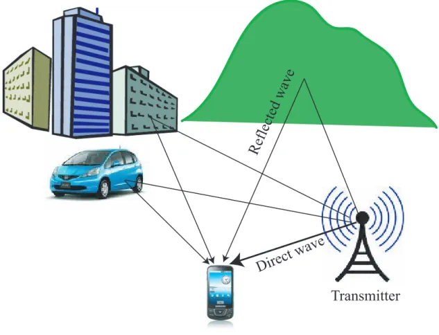
each OFDM symbol. The duration of the guard time is chosen in accordance with the multipath characteristics of the channel. To avoid the creation of ISI and inter-carrier interference (ICI), a cyclic extension should be longer than the length of channel delay spread. The price to be paid is transmission speed. For this reason, OFDM system de-signers always keep the guard time duration as short as possible. The multipath of the channel introduces delayed echoes of transmitted signal as shown in Fig. 2.2, where we can see that the received signal is consist of direct wave and reflected waves.

2.2 C

OMPARISON OF

FDM

AND

OFDM

Frequency division multiplexing (FDM) extends the concept of single carrier modula-tion by using multiple subcarriers within the same single channel. The total data rate to be sent in the channel is divided between the various subcarriers. Advantages of FDM include using separate modulation/ demodulation customized to a particular type of data,

(31)

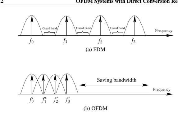
12 OFDM Systems with Direct Conversion Receiver Frequency Guard band Guard band Guard band f0 f1 f2 f3 (a) FDM Saving bandwidth Frequency f₀′ f₁′ f₂′ f₃′ (b) OFDM

Fig. 2.3. Comparison of spectral efficiency

or dissimilar data can be best sent using multiple modulation schemes. FDM systems usually require a guard band between modulated subcarriers to prevent the spectrum of one subcarrier from interfering with another. These guard bands lower the system’s effective information rate when compared to a single carrier system with similar mod-ulation. If the above FDM system had been able to use a set of subcarriers that were orthogonal to each other, a higher level of spectral efficiency could have been achieved. The guardbands that were necessary to allow individual demodulation of subcarriers in an FDM system would no longer be necessary. The use of orthogonal subcarriers would allow the subcarriers spectra to overlap, thus increasing the spectral efficiency. As long as orthogonality is maintained, it is still possible to recover the individual subcarriers signals despite their overlapping spectrums. This is the fundamental of OFDM. The comparison of spectral efficiencies of FDM and OFDM is shown in Fig. 2.3.

2.3 OFDM B

ASEBAND

S

YSTEM

M

ODEL

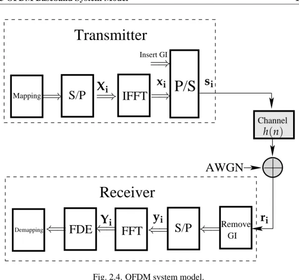
In OFDM systems, modulation and demodulation are implemented by using IFFT and FFT, respectively as shown in Fig. 2.4. At the transmitter side, after mapping and serial to parallel (S/P) conversion to the information data, IFFT will be performed. Then the

(32)

2.3 OFDM Baseband System Model 13

IFFT

S/P

Demapping

_FFT

S/P

Remove GI

Receiver

P/S

Mapping Insert GI

AWGN

Channel

Transmitter

FDE

x

_i

=

⇒

=

⇒

=

⇒

=

⇒

⇐=

Y

i

X

_i

h

(

n

)

⇐=

y

i

r

i

s

_i

Fig. 2.4. OFDM system model.

ith OFDM symbol with N length becomes

xi =FHXi, (2.2)

where, x_i = [x₀, x₁, . . . , x_N₋₁]T and X_i = [X₀, X₁, . . . , X_N₋₁]T correspond to the OFDM symbols in time and frequency domains respectively, andFH is an IFFT matrix as follows FH=√1 N         1 1 . . . 1 1 ej2Nπ . . . ej 2π(N−1) N .. . ... . .. ... 1 ej2π(N−1)N . . . ej 2π(N−1)(N−1) N         . (2.3)

(33)

Then, after GI insertion and parallel to serial (P/S) conversion, the OFDM signal is ready for transmitting. We assume that the signal pass through the channel, also the channel lengthL is less than GI length, and additive white Gaussian noise (AWGN) is added to

the received signal. Based on this assumption, after GI removal and S/P conversion, we can obtain theith received symbol yias follows

yi =hsi+zi, (2.4)

where,ziis an AWGN vector corresponding to theith symbol,

s_i =               xN−L .. . xN−1 x₀ .. . x_N₋₁               , (2.5)

and the channel matrixh is an N× (N+L−1)Toeplitz-like matrix

h =            h_L₋₁ . . . h₀ 0 . . . 0 0 . .. . .. . .. ... .. . . .. h_L₋₁ . . . h₀ . .. ... .. . . .. . .. . .. 0 0 . . . 0 h_L₋₁ . . . h₀            . (2.6)

Then, Eq.(2.4) can be rewritten as

y_i =h_cyclx_i+z_i, (2.7)

where,hcyc is a cyclic channel matrix as follows

h_cycl =               h0 0 . . . hL−1 . . . h0 .. . . .. . .. ... hL−2 . . . h0 hL−1 h_L₋₁ h_L₋₂ . . . h₀ ... 0 hL−1 hL−2 . . . h0 ... 0 . . . h_L₋₁ h_L₋₂ . . . h₀               . (2.8)

(34)

2.3 OFDM Baseband System Model 15

0

5

10

15

20

25

30

10

−4

10

−3

10

−2

10

−1

10

0

SNR [dB]

SER

QPSK

16QAM

64QAM

(35)

After performing FFT to the received symbol in Eq.(2.7), we have

Yi = Fhcyclxi+Fzi

= Fh_cyclFHXi+Zi, (2.9)

where,Zidenotes an AWGN vector in frequency domain, andF is FFT matrix as follows

F=√1 N         1 1 . . . 1 1 e−j2Nπ . . . e−j2π(N−1)N .. . ... . .. ... 1 e−j2π(N−1)N . . . e−j2π(N−1)(N−1)N         . (2.10)

SinceFh_cyclFH becomes diagonal matrix, from Eq.(2.9), we have

Yi =HdiagXi+Zi. (2.11)

Finally, the information can be recovered easily, by using frequency domain equalization (FDE) as follows

ˆ

X_i =H−_diag1 Y_i. (2.12)

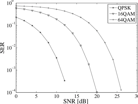
Figure.2.5 shows the results of bit error rate (BER) versus signal to noise ratio (SNR) to QPSK, 16QAM, and 64QAM respectively. We can see that the BER performance becomes worse with the increasing order of constellation.

2.4 ISI

IN

OFDM S

YSTEMS WITHOUT

GI

In this section, let us consider the effect of ISI in OFDM systems without GI. After passing through the channel, theith received OFDM symbol without guard interval can

be expressed as follows ri = ˙h·si−1,i+zi, (2.13) where, si−1,i =   si−1 si 

 is a 2N×1 vector consist of two consecutive transmitted

symbols andsi = [s0_i, s1_i, . . . , sN_i −1]T is an N×1 vector corresponding to ith symbol,

(36)

2.5 DCR Architecture 17 hx =               h₀ 0 . . . 0 .. . . .. . .. ... h_L₋₁ . . . h₀ . .. ... 0 hL−1 . . . h0 . .. ... .. . . .. . .. . .. 0 0 . . . 0 hL−1 . . . h0               , (2.14) ht =               0 . . . 0 hL−1 . . . h1 .. . . .. . .. . .. ... .. . . .. . .. h_L₋₁ .. . . .. 0 .. . . .. ... 0 . . . 0               . (2.15)

Obviously, these two matrices satisfy

hx+ht =hcycl, (2.16)

whereh_cycl is the “ideal” channel matrix, i.e., the matrix that results in a cyclic convo-lution between the transmitted signal and the channel. Then, we have

ri = hx·si+ht·si−1+zi. (2.17)

we can rewrite

ri =hcycl·si−ht·si+ht·si−1+zi, (2.18)

where, h_cycl ·s_i, ht ·si and ht ·si−1 represent the desired, ICI and ISI components

respectively. From Eq.(2.18), we can see that the desired signal is effected by ISI and ICI. This will result in severe performance degredation.

2.5 DCR A

RCHITECTURE

As indicated in introduction, the receivers can be classified to the superheterodyne re-ceiver and direct-conversion rere-ceiver (DCR). To better understand DCR architecture and

(37)

RF

filter filterIF

LPF

LO

₁

LO

₂

(

f

c

−

f

IF

)

(

f

IF

)

Fig. 2.6. Superheterodyne receiver.

RF

filter

LPF

LO

(

f

c

)

Fig. 2.7. Direct-conversion receiver.

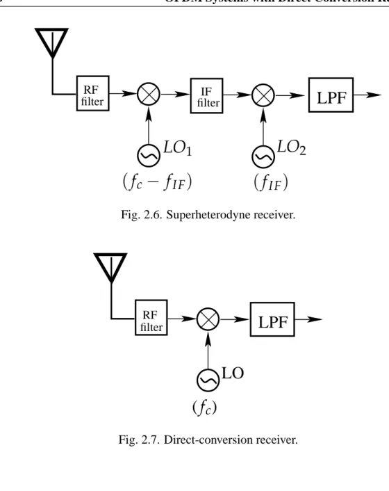
make clear the difference between DCR and superheterodyne receiver, we give simple diagrams of superheterodyne receiver and DCR respectively in Figs.2.6 and 2.7. As shown in Fig.2.6, superheterodyne receiver filters the received radio frequency (RF) sig-nal with carrier frequency fcand converts it to a lower intermediate frequency (IF) fIFby

mixing with an offset local-oscillatorLO₁ with frequency fc− fIF. Then, the resulting

IF signal is converted again byLO2 at an intermediate frequency fIF, and finally

base-band signal is obtained by using low pass filter (LPF). However, the signal amplification requires IF filters to be biased with large currents, causing substantial power dissipation. Furthermore, these filters need many off-chip passive components, adding to receiver size and cost.

(38)

2.6 Impairments Caused by DCR 19

The process of frequency translation to zero IF is called direct-conversion and is illustrated in Fig.2.7. Since IF is zero, the desired signal is translated directly to the baseband. Therefore, the direct-conversion receiver (DCR) architecture relaxes the se-lectivity requirements of RF filters and removes all IF analog components, thus a small-size, low-cost and low-power can be achieved. Due to these merits, DCR is an attractive receiver for wireless communication.

2.6 I

MPAIRMENTS

C

AUSED BY

DCR

Although DCR has many considerable merits, it leads to additional analog impairments such as CFO, DCO, and I/Q imbalance, which causes severe performance degradation of the system. In this section we will discuss these impairments in detail.

2.6.1 CFO Caused by DCR

CFO is mainly caused by the frequency mismatch between transmitter and receiver local oscillators (LO’s) as shown in Fig.2.9, where fc is carrier frequency, and△fc is the

fre-quency error. After downconversion, let us see the effect of CFO to the system. For the simpilicity, we just consider one block of OFDM symbols. The total system bandwidth

B is divided into N subcarriers, at a spacing of ∆ f = B/N. Then, the downconverted

received signal with CFO can be expressed as follows (see Appendix A)

d(k) = y(k)ej2πεkN , _(2.19) where, d(k) denotes thekth sample of downconverted signal, y(k)is baseband equiva-lent signal of received signalr(k), andε is the CFO normalized to the subcarrier spac-ing, which equals the actual CFO∆ f_c divided by the OFDM subcarrier spacing∆ f . As shown in Eq.(2.19), since the received samples are actually affected by the normalized CFOε, the normalized CFO is often called as CFO in CFO estimation, for the simplicity. Eq.(2.19) can be expressed by matrix form as

d=Γ(ε)y, (2.20)

where, the matrixΓ(ε)is corresponding to the CFO as

Γ(ε) = diag(1, ej2Nπε, ej4πεN , ej6Nπε, ..., ej 2πε(N−1)

N ). _(2.21)

This can be rewritten as

(39)

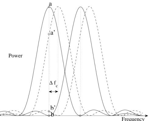
whereY = Fy. While CFO occurs, since OFDM spectrum will be shifted, the

orthog-onality between subcarriers should be distroyed. The effect of the CFO is shown in Fig.2.8, where the solid wave and the dashed wave indicate original OFDM spectrum and OFDM spectrum with the effect of CFO, respectively. In this figure, from the ob-servation point at a and b on the solid wave, we can see that subcarriers maintain its

orthogonality in original OFDM spectrum. However, from the observation point at a′

and b′ on the dashed wave, we can see that the orthogonality is distroyed with CFO

△fc, since the spectrum is shifted. Therefore, in OFDM systems, CFO compensation is

very important. 950 1000 1050 1100 1150 1200 1250 1300 1350 1400 ∆ f c Frequency Power

a

a’

b’

b

(40)

2.6 Impairments Caused by DCR 21 cos( 2π fc t) Upcon v ersion OFDM signal Base band Tx Rx

BPF

LPF

A/D

Q branch

LPF

A/D

I branch -sin( 2π ( fc + ∆ fc ) t) cos( 2π ( fc + ∆ fc ) t) Do wncon v ersion r ( t ) Fig. 2.9. Model of CFO.

(41)

2.6.2 I/Q Imbalance Caused by DCR

The I/Q imbalance is caused by the mismatched components between the in-phase (I) and quadrature-phase (Q) branches. Let us assume that the amplitude mismatch isg and

phase error isϕ. Based on this assumption, the mathematical model of I/Q imbalance is shown in Fig.2.10. In the figure, the received signal r(t), which is centered at fc with

bandwidthB, can be written as

r(t) =2Re[s(t)ej2π fct_{] =}_s₍_t₎_ej2π fct₊_s∗₍_t₎_e−j2π fct_, _(2.23) wheres(t) = sI(t) +sQ(t) is baseband equivalent signal ofr(t). The local oscilator

signalx_LO(t)with I/Q imbalance experessed by

xLO(t) = cos(2π fct)−jg·sin(2π fct+ϕ). (2.24)

This can be rewritten as follows

x_LO(t) = e j2π fct₊_e−j2π fct 2 −jg· ej(2π fct+ϕ) −_e−j(2π fct+ϕ) 2 = C1·e−j2π fct+C2·ej2π fct, (2.25) whereC₁ = 1+ge₂−jϕ andC₂ = 1−₂gejϕ.

As shown in Fig.2.10, the received signal r(t) is downconverted to baseband by mixing it with LO signalxLO(t). Therefore, the downconverted signal can be written as

r(t)·x_LO(t) = {s(t)ej2π fct₊_s∗₍_t₎_e−j2π fct}(_C

1·e−j2π fct+C2·ej2π fct)

= C₁s(t) +C₂s(t)ej4π fct₊_C

1s∗(t)e−j4π fct+C2s∗(t). (2.26)

Then, after passing through the low pass filter (LPF), the high frequency components of

C2s(t)ej4π fct andC1s∗(t)e−j4π fct are removed. Then the signal becomes

y(t) = LPF{r(t)x_LO(t)} = C₁s(t) +C2s∗(t), (2.27)

where y(t) = yI(t) +yQ(t), C1s(t) is desired part, C2s∗(t) is undesired part also

known as image part, which is caused by I/Q imbalance. In ideal case without I/Q imbalance, the second term C2s∗(t) should be zero. From Eq.(2.27), we can see the

(42)

2.6 Impairments Caused by DCR 23

LPF

I branch

Q branch

I/Q imbalance

r

(

t

)

−

g

· sin(

2 π f

c

t

+

ϕ

)

cos(

2 π f

_c

t

)

y

_Q

(

t

)

y

_I

(

t

)

Fig. 2.10. Model of I/Q imbalance.

2.6.3 DC Offset Caused by DCR

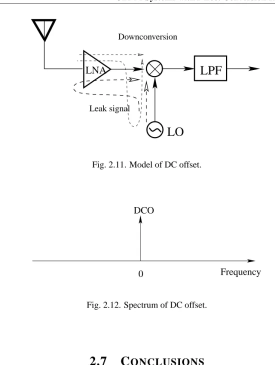
DC offset is induced by the self-mixing of leaking LO signal due to the imperfect iso-lation and is known as the most serious problem [2] of DCR. This offset appears in the middle of the downconverted signal spectrum, and may be larger than the signal itself. While DCO happens, the SNR at the detector input will be very low. The LO signal leaking from the antenna during receive mode may reflect off an external object and self-downconvert to dc in the mixer as shown in Fig. 2.11. Similarly, a large undesired near-channel interferer in the preselect filter passband may leak into the LO port of the mixer and self-downconvert to dc. In order to remove DCO, appropriate circuits is nec-essary at the receiver. For example, at the I branch in Fig.2.10, let us assume the leaking of LO signal is selfmixed at the mixer, and resuls in DCO. Then it can be expressed as

y(t) = cos(2π fct)·βcos(2π fct) = cos(4π fct)/2+β/2, (2.28)

whereβ denotes the leaking factor. Then after LPF, the second term β/2 is left as DCO. In the same way, we can obtain similar result for the Q branch. The spectrum of DCO is shown in Fig.2.12, where we can see that DCO corresponds to zero frequency.

(43)

LNA

Downconversion

LPF

LO

Leak signal

Fig. 2.11. Model of DC offset.

Frequency

0 DCO

Fig. 2.12. Spectrum of DC offset.

2.7 C

ONCLUSIONS

In this chapter, we introduced OFDM basis and the analog impairments caused by direct conversion receiver, such as CFO, I/Q imbalance and DCO. Moreover, we analyzed this impairments in detail and expressed by matrix form. In addition, we discussed the ISI problem in OFDM systems without GI, by using matrix form. This will help us to better understand the background knowledge discussed on this thesis.

(44)

C H A P T E R

3

Robust CFO Estimation in the Presence

of TV-DCO

O

FDM is known for its sensitivity to CFO, which is mainly caused by frequency mismatch between the transmitter and receiver local oscillators. Since the CFO destroys the orthogonality among subcarriers, the resulting inter-carrier interference (ICI) leads to severe performance degradation [41].

On the other hand, DCR has attracted a lot of attention in recent years, for its smaller size and lower cost over the traditional superheterodyne receivers. However, the price is the additional disturbances, such as DCO, I/Q imbalance, even-order distortion and flicker noise [4]. Among these, DCO, induced by the self-mixing associated with the unperfect isolation, is known as the most serious problem [2]. Obviously, the coexistence of the CFO and DCO is a critical problem in an OFDM DCR.

In the absence of DCO, the CFO can be estimated easily from the autocorrelation of periodic pilot (PP) [14, 26, 30, 40]. Considering DCO, several joint compensation schemes have been proposed in [7, 12, 15, 37], where DCO is assumed time-invariant. In practice, automatic gain control (AGC) is usually used to keep the received signal amplitude proper fixed level. Also, a high pass filter (HPF) is often employed in the DCR to reduce DCO [47]. Therefore, the gain shift in the low noise amplifier (LNA) will cause a TV-DCO [38], whose high frequency components may pass through the HPF. As a result, the ordinary CFO estimation in [7, 12, 15, 37] will be corrupted by the residual TV-DCO. Until now, there is only one CFO estimator taking the residual TV-DCO into account [25]. In this scheme, a differential filter is used to eliminate the residual TV-DCO, and then the CFO is estimated by the conventional

(45)

26 Robust CFO Estimation in the Presence of TV-DCO 10

t

9

t

8

t

7

t

6

t

5 4

t

3

t

2

t

1

GI2

T1

T2

10×0.8µs=8µs 2×0.8µs+2×3.2µs=8µs

STS

LTS

Fig. 3.1. IEEE 802.11a preamble.

based method. Since the differential filter increases the noise variance and the residual TV-DCO cannot be eliminated completely, this method will cause performance loss.

The purpose of this chapter is to develop a novel CFO estimation method in the presence of TV-DCO. As indicated in [25], the residual DCO at the output of the HPF has a linear property. Therefore, it can be approximated by a linear function. On the other hand, it has been shown in [15] that the CFO can be estimated independent of the time-invariant DCO, by exploring the periodicity of the pilot. Motivated by [15] and based on the linear property of the TV-DCO, we propose a PP-aided CFO estimator, which is able to remove the effect of TV-DCO during the CFO estimation process. After the CFO estimation, the residual TV-DCO can be obtained accordingly. Simulations confirm the effectiveness and superiority of the proposed estimator.

3.1 P

ROBLEM

F

ORMULATION

The pilot used for the joint estimation is the preamble of the IEEE 802.11a [1] shown in Fig.3.1. This preamble has a short training sequence (STS) and a long training sequence (LTS). The STS consists of ten identical K-samples repeated symbols t1,· · · , t10, and

LTS consist of two identical N-samples repeated symbols T₁ and T₂, where N = 64

andK =16. Every four repeated symbols of the STS can be treated as an N-subcarriers

OFDM symbol, which has only12 equally-spaced subcarriers loaded, see the generation

of the STS in [1]. When the channel is time-invariant during the preamble and the channel length is less than K, the received STS keeps its periodicity after discarding

the first symbol. This can be understood that the pattern of the loaded subcarrier in the received STS still is equally-spaced. We can partition IFFT matrixFHinto two matrices

W and V, corresponding to the loaded and unloaded subcarriers, respectively.

(46)

3.2 Conventional Method 27

(DCO)

(AWGN)

(CFO)

channel

x(n)

z(n)

d(n)

e

j2Nπεn

s(n)

h(n)

r(n)

Fig. 3.2. Mathematical model.

sample of the preamble after passing through the channel, ε is the CFO normalized to subcarrier spacing, d(n) and z(n) are the possible DCO and additive white Gaussian noise (AWGN), respectively.

In the absence of DCO, the received samplers(n)corresponding to the STS can be

written as

rs(n) =ss(n)ej

2πε

N n+z(n). _(3.1)

As mentioned above, we havess(n) = ss(n+K)forK≤n <9K. Then the normalized

CFO can be estimated by taking the autocorrelation of the STS as

ˆ ε= 4 2πarg{ 8

∑

m=2 K−1

∑

k=0 r_s∗(k+mK)rs(k+ (m+1)K)}, (3.2)

wherem is the index of the repeated symbols in the STS.

In the presence of a time-invariant DCOd, the received signal becomes rs(n) = ss(n)ej

2πε

N n₊d₊z₍n₎_. _(3.3)

In [7], it is known that the CFO estimation in Eq.(3.2) is biased. Hence, several PP-based joint estimation scheme have been proposed in [7, 12, 15, 37].

3.2 C

ONVENTIONAL

M

ETHOD

In practice, in order to keep the proper fixed level of the received signal, AGC circuits are usually employed [38]. In 802.11a WLAN systems, at the middle of STS, the AGC starts to adjust the gain of the received signal, which also changes the gain of DCO.

(47)

28 Robust CFO Estimation in the Presence of TV-DCO

The output of HPF

DCO Time 10 t 9 t t8 t7 t6 t5 4 t 3 t 2 t t1 GI2 T1 T2 GI Signal

r

₄

r

₃ STS LTS

⇒The gain of LNA changes from t₅

r

₂

r

₁

Fig. 3.3. Model of the residual TV-DCO.

On the other hand, a HPF is often used to eliminate DCO [47]. When DCO is time-invariant, a HPF is sufficient to remove the effect of DCO, then enables the CFO estimation in Eq.(3.2). However, the higher frequency components of the AGC-induced TV-DCO may pass through the HPF. In consequence, the CFO estimation will suffer from the residual TV-DCO. In [25], it has been shown that the residual DCO varies in a linear fashion, see the example given in Fig.3.3, where the LNA switches at the beginning of t5. Then, the authors propose to use a differential filter to counteract the

impact of the residual TV-DCO.

At the coarse CFO estimation stage, the STS is used, whose nth sample can be

written as

rs(n) = ss(n)ej

2πnε

N +d(n) +z(n), _(3.4) whered(n)denotes the residual TV-DCO. The received STS is passed through a differ-ential filter, and thenth sample of the differential filter’s output is given by:

r_sd(n) = rs(n)−rs(n−1) = s_sd(n)ej2πnεN ₊d_sd₍n_{) +}z_sd₍n₎_, _(3.5) where s_sd(n) = ss(n)−e−j 2πε N s_s(n−1), d_sd(n) = d(n)−d(n−1), z_sd(n) = z(n)−z(n−1).

(48)

3.3 Proposed Method 29

Asss(n)is a PP with a period ofK, so does ssd(n). Then the normalized CFO valueεˆ1

is estimated by replacingrs(n)withrsd(n)in Eq.(3.2).

At the fine CFO estimation stage, the obtainedεˆ₁is used to compensate the CFO in the LTS, which is also passed through the differential filter. Let r_ld(n) denote the nth

sample of the LTS after the differential filter and coarse CFO compensation. Since the LTS is a PP with a period ofN, the residual normalized CFO is calculated by

ˆ ε2= 1 2πarg{ N−1

∑

n=0 r∗_ld(n)r_ld(n+N)}. (3.6) Finally, the CFO estimate is given byεˆ=εˆ1+εˆ2.

3.3 P

ROPOSED

M

ETHOD

Compared Eq.(3.4) with Eq.(3.5), it is clear that the above mentioned CFO estimation still is biased by d_sd(n). Moreover, the noise variance is doubled, which also leads to performance loss. Here, by extending the method in [15], we will derive a novel CFO estimator, which can remove the effect of the TV-DCO completely. Similar to [25], we assume the LNA is switched at the beginning of t₅.

At the coarse estimation stage, without loss of generality, we can form two N×1

vectorsr1 andr2 from the received STS symbolst6, t7,· · · , t10, which are at a distance

ofK shown in Fig.3.3. Note that r₁andr2are the symbols corresponding to the sampling

range of t6−t9 and t7−t10, respectively. Since the TV-DCO is approximated by a

linear function ax+b, a denotes the ratio of variation, while b stands for the constant

component. Then,r₁andr₂can be expressed as

r1 = Γ(ε)Ss+ax1+b1N +z1, (3.7) r2 = ej 2πKε N Γ(ε)S_s+ax₂+b1_N +z₂, _(3.8) x1 = [0, 1, · · · , N−1]T, (3.9) x2 = [K, K+1,· · · , K+N−1]T, (3.10) where Γ(ε) = diag(1, ej2Nπε, . . . , ej 2πε(N−1) N ), _(3.11) Ss = [sT, sT, sT, sT]T, (3.12)

ands= [ss(0), ss(1),· · · , ss(K−1)]Tis a distortion free STS symbol,znis an AWGN

(49)

Then, in the absence of AWGN, we should have

ej2πKεN (r₁−ax₁−b1_N) = r₂−ax₂−b1_N. _(3.13) Thus, the CFO and DCO can be estimated as

(ε, â, ˆbˆ ) = argmin ˜ ε,ã,˜b ∥ r2−ej 2πK˜ε N _r₁−ã₍_x₂−ej2πK˜εN _x₁₎−˜b₍1−ej2πK˜εN ₎₁_N ∥2 . (3.14) This equation indicates a least squares problem for three unknown scalar. The optimal solution is given by      ej2πKˆεN â(1−ej2πKˆεN ) ˆb(1−ej2πKˆεN ) + âK     = [r1x11N]†r2=R. (3.15)

The first element ofR is given as

R(1) = 1 Gr H 1 Dr2, (3.16) D={x₁Tx11TN1N−xT11N1TNx1}IN +1N1TNx1xT1 −x11TN1Nx1T +x₁x₁T1N1TN −1NxT1x11TN, (3.17)

whereIN is the N×N identity matrix, and

G = rH₁ r1x1Tx11TN1N +rH1 x1x1T1N1TNr1 + xT₁r1rH1 1N1TNx1−rH1 1N1TNr1x1Tx1 − rH₁ r1x1T1N1TNx1−rH1 x1x1Tr11TN1N = rH₁ Dr1. (3.18) Then we have r₁HDr2 =ejϕ˙SHs D ˙Ss+a ˙SHs Dx2+b ˙SHs D1N +aejϕxT₁D ˙Ss+a2xT₁Dx2+abxT1D1N +bejϕ1T_ND ˙Ss+ab1TNDx2+b21TND1N+Rz, (3.19) where Rz =ejϕzH1 D ˙Ss+azH1 Dx2+bzH1 D1N +zH₁ Dz₂+ ˙SH_s Dz₂+axT₁Dz₂+b1T_NDz₂, (3.20)

(50)

3.3 Proposed Method 31

and ˙Ss =Γ(ε)Ss,ϕ= 2πKε_N .

It can be proved that the matrix D is symmetric, D1N = 0N, Dx1 = 0N, and

Dx2=0N (see Appendix B for the proof), where0N is anN×1 all 0 vector. Then we

have R(1) = 1 Gr H 1 Dr2 = 1 G(e jϕ_˙SH s D ˙Ss+ ˙Rz), (3.21) where ˙Rz =ejϕzH1 D ˙Ss+zH1 Dz2+ ˙SHs Dz2. (3.22)

Obviously, inR(1), all terms containing DCO parameters a and b are removed.

Conse-quently, we obtain a CFO estimate independent of TV-DCO as

ˆ

ε1=

4

2πarg{R(1)}. (3.23)

At the fine estimation stage,εˆ₁ is used to compensate the CFO in the received LTS symbols. Let the vectorsr₃andr₄express the received two LTS symbols, which can be written as

r3 = Γ(ε)Sl+ax3+b1N +z3, (3.24)

r₄ = ej2πεΓ(ε)S_l+ax₄+b1_N +z₄, (3.25)

x3 = x1+Q1N, (3.26)

x4 = x3+N1N, (3.27)

where S_l is a distortion-free LTS symbol, and Q is the distance between r1 and r3.

Similarly, the initial phase offset of the CFO is absorbed into the channel. After the CFO compensation, we have

˜r₃ = Γ(εˆ₁)H{Γ(ε)S_l+ax₃+b1_N +z₃}, (3.28)

˜r4 = e−j2πˆε1Γ(εˆ1)H{ej2πεΓ(ε)Sl+ax4+b1N +z4}. (3.29)

Using the same approach at coarse estimation stage, we have

     ej2π(εˆ−εˆ1) ae−j2πˆε1₍₁−_ej2πˆε₎ e−j2πˆε1{_b₍₁−_ej2πˆε_{) +}_aN}     = [˜r3 ˜x3 ˜1N]†˜r4,

where ˜x3 =Γ(εˆ1)Hx3and ˜1N =Γ(εˆ1)H1N. Henceεˆ2=εˆ−εˆ1can be obtained by

ˆ

ε2= 1

(51)

Table 3.1. Computational complexity Proposed Differential

Subtraction - N+K−1

Addition N× (N+1) N

Multiplication N× (N+1) N

where ˜R(1)indicates the first element of the3×1 vector[˜r3 ˜x3 ˜1N]†˜r4. Finally, the fine

CFO estimation is given by

ˆ

ε=εˆ₁+εˆ₂. (3.31)

On the other hand, the residual TV-DCO can be estimated by usingε. For ˆεˆ ̸=0, the

parametera of the residual TV-DCO can be calculated from Eq.(3.15) as

ˆa = R(2) (1−ej2πKˆεN )

. (3.32)

Then, usingε and ˆa, we haveˆ

ˆb = R(3)−ˆaK (1−ej2πKˆεN )

. (3.33)

However, this method cannot work when theε is close to zero. As mentioned in Sectionˆ

3.1, since the matrixV consists of the columns of the IFFT matrix that correspond to the

unloaded subcarriers, we knowVHSs =0. In the absence of noise, we have

VHΓ(εˆ)Hr₁ =aVHΓ(εˆ)Hx₁+bVHΓ(εˆ)H1N. (3.34)

Therefore, using least square method, we can obtain ˆa and ˆb as   ˆa ˆb  = [A B]†VHΓ(εˆ)Hr1, (3.35) whereA =VHΓ(εˆ)Hx1andB=VHΓ(εˆ)H1N.

The computational complexity of the coarse estimation is shown in Table.3.1. The similar result can be found for the fine estimation. From the comparison result, we can see that the proposed method needs more calculation than the differential filter method.

大阪府立大学 学術情報リポジトリ

Analog Impairments Compensation in OFDM

Direct-Conversion Receiver

著者

Umut Yunus

内容記述

学位授与大学: Osaka Prefecture University(大阪

府立大学), 学位の種類: 博士(工学), 学位記番号:

論工第1245号, 学位授与年月日: 2010-03-31, 指導

教員: 山下勝己.

Analog Impairments Compensation in

OFDM Direct-Conversion Receiver

Umut Yunus

February 2010

Analog Impairments Compensation in

OFDM Direct-Conversion Receiver

A dissertation submitted to the

Graduate School of Engineering

in partial fulfillment of

the requirements for the

degree of Doctor of Engineering

Umut Yunus

Sakai, February, 2010

Acknowledgments

W

Contents

List of Figures

List of Tables

List of Acronyms

C H A P T E R

1

Introduction

T

1.1

T

ENDENCY OF

W

IRELESS

C

OMMUNICATION

S

YSTEMS

1.2

T

HE

R

ECEIVER

A

RCHITECTURE

1.2.1

Superheterodyne Receiver

1.2.2

Direct-Conversion Receiver

1.3

A B

RIEF

R

EVIEW OF

OFDM-DCR

1.3.1

CFO

1.3.2

DCO and I/Q Imbalance

1.3.3

Time-Varying DCO Caused by AGC

1.4

I

NTER

-S

YMBOL

I

NTERFERENCE

C

ANCELLATION

IN

OFDM S

YSTEMS WITHOUT

G

UARD

I

大阪府立大学　学術情報リポジトリ

_FFT