132
Deformation
of a
renormalization-group
equation
applied
to infinite-Order
phase
transitions
埼玉医科大学 物理学教室 向田 寿光(Hisamitsu Mukaida)
Department of Physics,
Saitama
Medical College$\mathrm{m}\mathrm{u}\mathrm{k}\mathrm{a}\mathrm{i}\mathrm{d}\mathrm{a}\mathrm{Q}\mathrm{s}\mathrm{a}\mathrm{i}\mathrm{t}\mathrm{a}\mathrm{m}\mathrm{a}-\mathrm{m}\mathrm{e}\mathrm{d}$
.
$\mathrm{a}\mathrm{c}$.
jpABSTRACT
By adding
a
linear term toa
renormalzation-groupequationina
systemexhibitinginfinite-order phase transitions, asymptoticbehavior ofrunning coupling
constants are
derived inan
algebraic
manner.
A benefit
of this method is presented explicitly using severalexamples.I. INTRODUCTION
Renormalzation-group (RG) technique is
one
of the most powerfulmethods forinvesti-gating
critical
phenomena instatistical
physics[l]. In general,RG
transformation (RGT)consists of a coarse graining and a rescaling. It reduces many-body effects in a statistical
model to
an
ordinary differential equation of coupling constants. The differential equationis
called
theRG
equation (RGE), and has generally the following form:$\frac{dg}{dt}=V(g)$ , (1)
where $g=$ $(g_{1}, \ldots,g_{n})$,
a
collection of coupling constants dependingon
$t$, and $t=\log L$with $L$ givingthe length scale of the
coarse
graining in the $\mathrm{R}\mathrm{G}$.One
obtainsa
beta function$V(g)=$ ($V_{1}(g)$, $\ldots$,Vn(g)) by applying the
RGT
explicitly toa
statistical model. Wecan
derive universal exponents that characterize critical phenomena from asymptotic behavior
of solutions of Eq. (1) for large $t$
.
Since the asymptotic behavioris determinedby vicinity of
a
fixed point$g^{*}$, linearizationof$V(g)$
about
$g^{*}$ iseffective
enoughtoobtain the exponents.For
example, ina second-Order
phase transition, the
correlation
length4
typically behavesas
$\xi=$const./lT $-T_{c}|^{\nu}$, (2)
where $\nu$ is the correlation-length exponent and $T$ is
a
parameter specifyinga
state
ina
statistical
model (e.g., the temperature). In the language of $\mathrm{R}\mathrm{G}$, $T$ parametrizes initial133
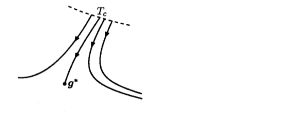
FIG. 1: Typical RG trajectories near a phase transition. As $T$ Changes, an initial value
moves
onthe dashed line. The trajectory with $T=T_{c}$ is absorbed into the fixed point$g^{*}$
.
values
of
RGE.
The trajectory starting from the initial value at $T=T_{\mathrm{c}}$ isabsorbed
intothe fixed point. Other trajectories approach $g^{*}$
once
but leave the fixed point subsequently,as
shown in Fig. 1. This implies that it takes longer for $g$ to leave the fixed pointas
$T$approaches $T_{c}$
.
Let $\overline{t}$
be time satisfying $|g(?)-g^{*}|\sim \mathrm{O}(1)$. Then the correlation length
4
is related to $\overline{t}$by the following formula[l]:
$4=$ const, $\mathrm{x}e^{\overline{t}}$
.
(3)
Therefore, if the scaling matrix $M(g^{*})$, where
$M_{j} \dot{.}(g^{*})\equiv\frac{\partial V_{i}}{\partial g_{j}}(g^{*})$ (4)
has
a
unique positive eigenvalue $\alpha$, $t$ behavesas
$|g(\overline{t})-g^{*}|\sim|a(7)$$|ea\overline{t}$
’ (5)
as
$\overline{t}arrow\infty$.
Here $a(T)$ isan
initial value parametrized by $T\mathrm{t}$ Expanding $a(T)$ about $T=T_{c}$,we
have$\overline{t}\sim|T-T_{c}|^{-1/a}$ (6)
as
$\overline{t}arrow\infty$.
From
Eqs.(2), (3) and (6),we
get$\nu=\frac{1}{\alpha}$
.
(7)In
this way,
we
do not need to findan
explicit solution ofnonlinearRGE
(1).On
the other hand, in thecase
of infinite order phase transitions,4
has the followingessential
singularity:134
where $\sigma$ is a universal exponent and $A>0$ is
a non-universal
constant. Such behavior isobserved
when all the couplingconstants are
marginal, i.e. when thecanonical
dimensionsof the coupling
constants
are zero
at $g^{*}$.
Since
the linear term in $V(g)$ is proportional tothe
canonical
dimensions of$g$, $M_{ij}(g^{*})=0$ for all$i$and
$j$ in thecase
of infinite-Order phasetransitions.
The
essential
singularity in Eq.(8) isunderstood
from the following simple example:$\frac{dg(t)}{dt}=(g-g^{*})^{2}$
.
(9)$\frac{dg(t)}{dt}=(g-g^{*})^{2}$
.
(9)The
solution
starting from $a(T)$ at $t=0$ is$g(t)-g^{*}= \frac{1}{\frac{1}{a(T)-g^{*}}-t}$
.
(10)We
assume
that $a(T_{c})=g^{*}$ and that$a(T)=g^{*}+b(T-T_{c})+\mathrm{O}((T-T_{c})^{2})$
If $\overline{t}$satisfies
$|g(t\mathrm{J}$ $-g^{*}|=1,$
then
$\xi=$ const,$\exp\overline{t}\sim$const,$\exp(\frac{1}{|b(T-T_{c})|})$
,
(13)as
$Tarrow T_{e}$.
Thus $\sigma=1$and
$A=1/|b|$ in this example.One
finds that the essentialsingularity originates from the
rational
form ofthe solution Eq.(10). Note that $A$ dependson a
functional form of$a(T)$ while $\sigma$ doesnot,as
longas
we
do not consider the exceptionalcase:
$b=0.$Since
the scaling matrix $M(g^{*})$ vanishes inan
infinite-Order phase transition, we cannotextract $\sigma$ from the usuallinearization, in contrast to
a
second-Orderone.
As we have shownin the aboveexample, explicit solutions
were
traditionally$\mathrm{r}.\mathrm{e}$quiredin thecase
ofan
infinite-order phase transition
such
as
theBKT
phase transition[2].This difficulty has been recently
overcome
in Ref.[3], wherean RG
forRGE
(1) is usedfor deriving asymptotic behavior of solutions. A general idea of $\mathrm{R}\mathrm{G}$, applied
as a
tool forasymptotic analysis of non-linear
differential
equations, is developed in Refs.$[4, 5]$.
In this report,
we
present another method. Namely,we
derive $\sigma$ from the followingdeformed
RGE:135
where $\epsilon$is
a
real number but not necessarilysmall.As
we
willsee
in the next section,the RG
equation (22) for the
RGE
(1) hasa
complicated form compared with thedeformed
RGE.Hence, using the deformed
RGE
makes derivation ofthe critical exponent simple. Anotherbenefit of this approach is
as
follows: suppose thatan
infinite-Order phase transitionoccurs
when the spatialdimensions of theoriginalstatisticalmodel
are
$d_{c}$. Then,the deformedRGE
can
bederived
whentheyare
$d_{c}-\epsilon$, underthe condition that all the coupling constantshave
a
common
canonicaldimension. This conditionis satisfiedby variousfield-theoretical
models,e.g., an effective
theory of antiferromagnets[6],a
model containing severalgauge
fields[7],a
modeldescribing true self-avoiding random walks[8], and
a
model of nematic elastomers[9].In Ref.[9], inffared asymptotic behavior in$d_{c}$ dimensions and$d_{c}-\epsilon$ dimensions
are
analyzedseparately because of the problem of the vanishing scaling matrix explained above. Our
method enables
us
toobtainuniversal quantities in both casessimultaneously. We willshowthis advantage in the last example of
Sec.IV.
$\mathrm{I}\mathrm{I}$
.
RGE FOR RGEHere
we
summarize the results ofRef.[3] that will be used later. We consideran RGE
(1)for infinite-Order phase transitions that
are
controlled bya
fixed point $g’$. In what follows,we
put $g^{*}=0$ for convenience. Suppose that we have obtained $V(_{\mathrm{j}}g)$ by thelowest-Order
perturbation. Since linear terms vanish in infinite-Order phase transitions, components of
$V(g)$
are
quadratic in $g$. Hence the scaling property$V(kg)=k^{2}V(g)$ (15)
holds in this
case.
In order to evaluate the asymptotic behavior of a solution of Eq.(l),
we
define anotherrenormalization group
on
an
$n-1$ dimensional sphere. We denote the solution $g$ of Eq.(l)withthe initial condition $a_{0}=( 1)\cdots,$$a_{0n})$
as
$g(t, a_{0})$, (16)
namely, $g(0, a_{0})=a_{0}$
.
The function $\mathrm{e}\mathrm{T}\mathrm{g}(\mathrm{e}\mathrm{T}\mathrm{t})\mathrm{a}\mathrm{o})$ isa
solution of theRGE
(1)as
well,because
of its scale invariance. Let $S$be
the $n-1$dimensional
spherewhose center
is at136
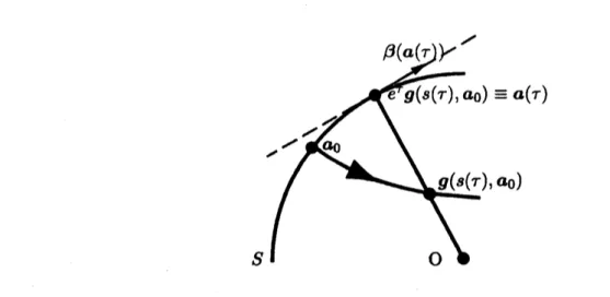
FIG. 2: Illustration for
74
andthebeta functiondefined inEq.(22). For simplicity, wetake $n=2.$Dashed line represents the tangent space at $\mathrm{a}(\mathrm{r})\in S$
.
$\mathcal{R}_{\tau}$ : $Sarrow S$
as
follows:$\mathcal{R}_{\tau}a_{0}\equiv e^{\tau}g(s(\tau), a_{0})\equiv a(\tau)$
.
(17)Using Eq.(15),
one
finds that $\mathcal{R}_{\tau}$ hasa
semi-group property:$\mathrm{R}$ $+’=\mathcal{R}_{\eta}0\mathcal{R}_{\eta}$
.
(18)The meaning of
74
isas
follows: first, choose $\mathrm{r}$.
Thenmove
$a_{0}$ along the solution $g(t, \mathrm{a}\mathrm{o})$during the time $s(\tau)$
.
Here $s(\tau)$ is determined by the condition $g(s(\tau-), a_{0})e^{\tau}\in S.$See
Fig.2.
Next let
us
derive the beta function of$\mathcal{R}_{\tau}$.
Notingthat $V(g)$ is quadratic,we
have$\frac{da}{d\tau}=a+e^{\tau}V(g(s, a_{0}))\frac{ds}{d\tau}$
$=a+e^{-\tau}V(a) \frac{ds}{d\tau}$
.
(19)The length-preserving condition
$a \cdot\frac{da}{d\tau}=0$ (20)
leads to the following differentialequation for $s(\tau)$:
$\frac{ds}{d\tau}=-\frac{e^{\tau}a_{0}^{2}}{a\cdot V(a)}$ (21)
with the initial condition $s(0)=0.$ Inserting Eq.(21) into Eq.(19),
we
obtain the betafunction for
$\mathcal{R}_{\tau}$.
137
Note
that $\beta$can
be writtenas
$\mathrm{d}(a)=-\frac{a_{0}^{2}}{a\cdot V(a)}P(a)V(a)$, (23)
where $P$ is the $n\mathrm{x}$ $n$matrix that projects $V(a(\tau))$ onto the tangent space at $a(\tau)\in S:$
$P_{1;}(a) \equiv\delta_{ij}-\frac{a_{i}a_{j}}{a_{0}^{2}}$
.
(24)Since
$\mathrm{d}$$(a)$ is perpendicularto
$a$,
a
solution of
thenew
RGE
is restrictedon
S.
on
toducing the polar coordinates $\{\theta_{\alpha}\}_{1\leq\alpha\leq n-1}$
on
$S$ and the corresponding orthonormal basis,$\overline{e}_{\alpha}\equiv f_{\alpha}(a)^{-1}\frac{\partial a}{\partial\theta_{\alpha}}$, $\mathrm{f}_{a}(a)\equiv|\frac{\partial a}{\partial\theta_{\alpha}}|$ , (25)
we
can
expand /3(a)as
$n-1$
$\beta$$(a)=$ $\mathrm{p}$$\sqrt{}^{\sim}\alpha(a)\tilde{e}_{\alpha}$
.
(23) $\alpha=1$The
new
RGE
is representedas
$\mathrm{g}$ $(a)=f_{\alpha}^{-1}(a)\sqrt{}^{\sim}\alpha(a)$ (27)
in the polar-coordinate representation.
It is easily found that $a^{*}\in S$ is a fixed point of the new RGE (22) if $g(t, a^{*})$ is
a
straight flow line. In particular,
a
fixed pointon
an
incoming straight flow line satisfying$a^{*}\cdot V(a^{*})<0$plays
an
importantrole,because
trajectoriesnear
this fixedpoint correspondto trajectories of Eq. (1) approaching $g^{*}$
.
Unlike the original RGE, thenew
RGE
can
belinearized
about $a^{*}$.
In Ref.[3], it isshown
that the scaling matrix of thenew
RGE
$\mu_{a\beta}(a^{*})\equiv f_{\alpha}^{-1}(a^{*})\frac{\partial\beta_{\alpha}}{\partial\theta_{\beta}}(a^{*})$ (28)
plays
a
similar role to$M(g^{*})$ in theoriginalRGE
describinga second-Orderphasetransition.Namely, if thematrix $\mu(a^{*})$ has
a
unique positive eigenvalue $\lambda$, in whichtypical trajectoriesof theoriginal
RGE are
as
in Fig. 3 (a),we can
observe divergence of the correlationlengthby one-parameter tuning and
$\sigma=\frac{1}{\lambda}$ (29)
in Eq. (8).
On
theother
hand, if all the eigenvaluesof
$\mu(a^{*})$are
negative,where
typicaltrajectories
are
in Fig.3
(b), $g(t, a_{0})$behaves
as
plays
a
similar role to$M(g^{*})$ in theoriginalRGE
describinga second-Orderphasetransition.Namely, if thematrix $\mu(a^{*})$ has
a
unique positive eigenvalue $\lambda$, in whichtypical trajectoriesof theoriginal
RGE are
as
in Fig. 3(a),we can
observe divergence of the. correlationlengthby one-parameter tuning md
$\sigma=\frac{1}{\lambda}$ (29)
in Eq. (8).
On
theother
hand, ifaU
the eigenvaluesof
$\mu(a^{*})$are
negative,where
typicaltrajectories
are
in Fig. 3(b), $g(t, a_{0})$behaves
as
138
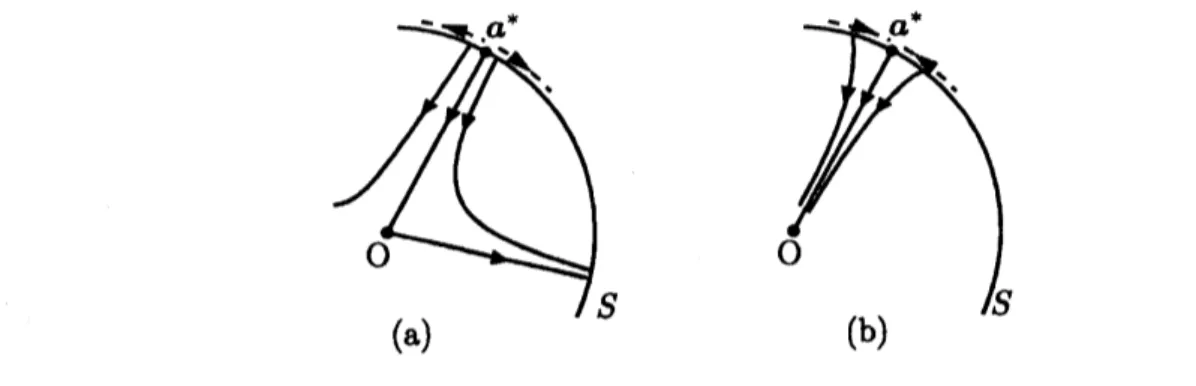
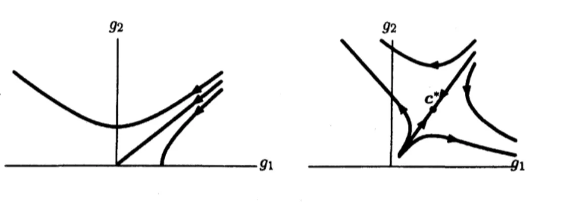
FIG. 3: Schematic trajectories of RGE. The solid lines are for the original RGE (1), while the
dashed lines arefor the new RGE (22) defined on $S$
.
Here (a) is the casewhere a unique positiveeigenvalue exists in$\mu(a^{*})$
.
(b) is thecase
where all the eigenvalues of$\mu(a^{*})$ axe negative.In this formula, $e^{*}\equiv a^{*}/a_{0}$ and $C(g)$ is
defined
by the relation$C(g)|g|^{3}=-g$, $V(g)$
.
(31)The asymptotic behavior in Eq. (30) is important for investigating finite-size scaling in
a
statistical system for example.
III. DEFORMED RGE
Next,
we
consider the deformed RGE (14), putting $g^{*}=0.$ Wecan
take $\epsilon>0$ withoutloss of generality. A fixedpoint $c^{*}$ of the
deformed RGE
solves$\overline{V}(c’)$ $=\epsilon c^{*}+V(c^{*})=0.$ (32)
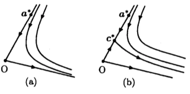
A key feature of the deformed
RGE
is that $c^{*}$ in Eq. (32) anda
fixed point $a^{*}$of
thenew
RGE
(22)on
an
incoming straight flow line hasone-tO-One correspondence via$a_{0}*$
$a^{*}=\mathrm{C}^{*}C$ (33)
as
depicted in Fig. 4. Writing $V(g)$as
$V(g)= \sum_{\alpha=1}^{n-1}\tilde{V}$
m
(g)$\tilde{e}_{\alpha}+\tilde{V}_{n}(g)\tilde{e}_{n}$, (34)where
$\tilde{e}_{n}\equiv g\int g,$we
havethe
deformed RGE
inthe
polarcoordinates:
$\frac{d\theta_{\alpha}}{dt}(g)=f_{a}^{-1}(g)\tilde{V}_{\alpha}(g)$
139
FIG. 4: (a) Schematic trajectories for the originalRGE. (b) Those for the deformed RGE.
Expanding the aboveformula about thefixedpoint $c^{*}$,
we
have the following scaling matrixIff$(c^{*})$: $\overline{M}_{\alpha\beta}(c^{*})=f_{\alpha}^{-1}(c^{*})\frac{\partial\overline{V}_{a}}{\partial\theta_{\beta}}(c^{*})$ $\overline{M}_{\alpha n}(c^{*})=f_{\alpha}^{-1}(c^{*})\frac{\partial\tilde{V}_{a}}{\partial g}(c^{*})$ $\overline{M}_{na}(c^{*})=\frac{\partial\tilde{V}_{n}}{\partial\theta_{\beta}}(c^{*})$ $\overline{M}_{nn}(c^{*})=(\epsilon+\frac{\partial\tilde{V}_{n}}{\partial g}(c^{*}))$ , (36)
where $\alpha$ and $\beta$
run
from 1 to$n-$ l. Since $V_{\alpha}(g)$ is
a
component perpendicular to$g$,
one
finds that $\tilde{V}_{a}(kc^{*})=0$ for all $k$ with the help ofEqs.(15) and (32). Thismeans
that$\partial_{g}\tilde{V}_{a}(c^{*})=0.$
On
the otherhand, $\partial_{g}\overline{V}_{n}(c^{*})=2\tilde{V}_{n}(c^{*})/g^{*}=$ -2e because$\tilde{V}_{\mathrm{n}}(g)$ is quadraticin $g$
.
Therefore,$M_{an}=0,$ $M_{nn}=-\epsilon$ (37)
in Eq. (36). Furthermore,
we can
rewrite $\overline{M}_{\alpha\beta}(c^{*})$ in terms of $\mu_{\alpha\beta}(a^{*})$.
In fact, $\mu(a^{*})$ inEq. (28) is written
as
$\mu_{\alpha\beta}(a^{*})=f_{\alpha}^{-1}(a^{*})\frac{1}{C(a^{*})a_{0}}\frac{\partial V_{a}}{\partial\theta_{\beta}}(a^{*})$
.
(38)Employing the following scaling properties:
$C(kg)=C(g)$
$f_{a}(kg)=kf_{\alpha}(g)$
140
we
get$\overline{M}_{\alpha\beta}(c^{*})=\epsilon\mu_{\alpha\beta}(a^{*})$
.
(40)Eqs.(37) and (40) shows that
-f
$(c^{*})$ hasa
form of$\overline{M}(c^{*})=$ $(\begin{array}{ll} 0 \vdots 0*\epsilon\mu(.a^{*}..)*-\epsilon\end{array})$ (41)
$|$
0
..
$\cdot$0
$*$ $\cdot$.
.
$*$ $|$ $-\epsilon$ $|$inthepolarcoordinates. Itreadilyfollows fromthisformula that $M(c^{*})\tilde{e}_{n}=-\epsilon e\sim n$
.
Thuswe
can
derive all the eigenvalues of$\mu(a^{*})$ from $\overline{M}(c^{*})$ by removing $-\mathrm{c}$, which is the eigenvaluecorresponding to the eigenvector $\tilde{e}_{n}$
, from
the setof
the eigenvaluesof
If(c’), and, bymultiplying by $1/\epsilon$, theremaining eigenvalues. Further, if all the eigenvalues of $\overline{M}(c^{*})$
are
negative, $g(t, a_{0})$
behaves
as
$g(t, a_{0}) \sim\frac{1}{C(a^{\mathrm{s}})t}e’=\frac{1}{\epsilon t}c$’, (42)
according to Eq. (30) and the scaling property of $C(a^{*})$ in Eq. (39)
$\mathrm{I}\mathrm{V}$
.
EXAMPLEHere
are
several
examples.The
first example is taken from the $\mathrm{t}\mathrm{w}\triangleright$imensional
classicalXY
mOde1[2]. Here, the beta function $V(g)$ is givenas
$V(g)=$ $(\begin{array}{l}-g_{2}^{2}-g_{1}g_{2}\end{array})$ , (43)
for$g_{1},g_{2}>0.$ The deformed RGE has the fixedpoint $c’=(\epsilon, \epsilon)$. The scalingmatrix $M(c^{*})$
of the
deformed RGE
is easily computed interms of the cartesian coordinatesas
$\overline{M}(c^{*})=$ $(\begin{array}{ll}\epsilon -2\epsilon-\epsilon 0\end{array})$ (44)
It has the eigenvalues $-\epsilon$
and
$2\mathrm{e}$.
Employing Eq. (29),we
get141
FIG. 5: (a) Schematic trajectories for the original RGE of the XY model. (b) Those for the
deformed RGEof theXYmodel.
which is
a
well-known result. Aswe
have explained in the previous section, the othereigenvalue, $-\mathrm{c}$, alwaysappears in
a
deformedRGE
(14),which correspondsto theeigenvector$c^{*}/c^{*}$
.
The next example is the RGE in
a
one
dimensional quantum spin chain, studied by Itoiand Kato[10]; it is defined by
$V(g)=$ $(\begin{array}{l}g_{1}(Ng_{1}+2g_{2})-g_{2}(2g_{\mathrm{l}}+Ng_{2})\end{array})$ (46)
The deformed
RGE
has the following three nontrivial fixed points:$c_{1}^{*}=(- \frac{\epsilon}{N}$,$0$
),
$\mathrm{c}_{2}^{*}=(0,$$\frac{\epsilon}{N})$ , $c_{3}^{*}= \frac{\epsilon}{N-2}(-1,1)$.
(47)The corresponding scaling matrices
are
$\overline{M}_{1}=$
$(\begin{array}{ll}-\epsilon -\frac{2\epsilon}{N}0 \underline{N}\pm\underline{2}N\epsilon\end{array})$:
$\overline{M}_{2}=$
$(\begin{array}{ll}\underline{N}\pm\underline{2}N\epsilon 0-\frac{2\epsilon}{N} -\epsilon\end{array})$ ,
$\overline{M}_{3}=$ $(\begin{array}{ll}\frac{N\epsilon}{2-N} \frac{2\epsilon}{2-N}\mathrm{t}_{\frac{2\epsilon}{2-N}}\prime \frac{N\epsilon}{2-N}\end{array})$
(48)
The eigenvalues of those matrices are, respectively,
$\frac{N+2}{N}\epsilon$, $\frac{N+2}{N}\epsilon$
,
md $\frac{2+N}{2-N}\epsilon$, (49)up
tothe
common
eigenvalue $-\epsilon$.
The
other eigenvaluesdivided
by $\epsilon$are
equal tothoseof
the scaling
matrices
derivedffom the
new
RGE
(22),which is computedin Ref.[3]. It should142
in $2-\epsilon$ and l-e dimensions respectively. However, the derivation presented here is much
simpler
than
the method using Eq.(22).The lastexample isthe
RGE
ina
field-theoretical model fornematic elastomers, proposedin Ref.[9]. In contrast to the previous examples, the deformed
RGE
is obtained exactly in$3-\epsilon$ dimensions with
$V(g)= \frac{-1}{8(4g_{1}+g_{2})}$ $(\begin{array}{l}g_{1}(40g_{1}^{2}+68g_{1}g_{2}+\mathrm{l}3g_{2}^{2})2g_{2}(4g_{1}^{2}+32g_{1}g_{2}+7^{2}g_{2})\end{array})$ (50)
Although $V(g)$ is not quadratic polynomial,
our
result is applicable becauseall
we
need
Although $V(g)$ is not quadratic polynomial,
our
result is applicable becauseall
we
need
$g_{1}$
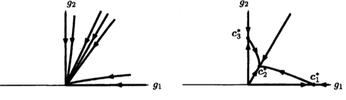
FIG. 6: (a) Schematictrajectories for the original RGE of the model of nematic elastomers. (b)
Those for the deformed RGE of the model of nematic elastomers.
to applythe present method isthe scaling property of$V(g)$, Eq. (15). The deformed
RGE
has the three fixed points
$c_{1}^{*}=( \frac{4\epsilon}{5}$,$0$
)
$)$
$\mathrm{c}_{2}^{*}=(\frac{4\epsilon}{59},$$\frac{32\epsilon}{59})’$. $c_{3}^{*}=(0,$ $\frac{4\epsilon}{7}$
)
(51)One can check that the scaling matrices have the following respective eigenvalues
$4\mathrm{c}/5$, $-4\mathrm{e}/59$,
and
$\mathrm{e}/14$ (52)in
addition to
thecommon
eigenvalue $-\mathrm{e}$.
Nowwe
turn to thecase of
justthree dimensions.
If $g_{1},g_{2}>0,$ infrared behavior of
a
system is governed by the fixed point $\mathrm{c}_{2}^{*}[9]$.
Since
theeigenvalue at $c_{2}^{*}$ is negative, $g(t, a_{0})$ behaves
as
$g(t, a_{0}) \sim\frac{1}{\epsilon t}c_{2}^{*}=\frac{1}{t}(\frac{4}{59},$$\frac{32}{59})$ (53)
143
V. SUMMARY
We have shownhow to derive asymptoticbehavior of
a
solution of RGE forinfinite-Order
phase transition, by adding
a
linear term to this RGE. This methodcan
allowus
to applya
result of the $\epsilon$ expansion to thecase
where $\epsilon=0.$[1] K. G. Wilson and J. Kogut, Phys. Rep. $12\mathrm{C}$, 75 (1974).
[2] V. L. $\mathrm{B}\mathrm{e}\mathrm{r}\mathrm{e}\mathrm{z}\mathrm{i}\mathrm{n}\mathrm{s}\mathrm{k}\mathrm{i}\check{\mathrm{i}}$, Zh.
\’Eksp.
Teor. Fiz. 59, 907 (1970) [Sov. Phys. JETP 32, 493 (1971)];
J. M. Kosterlitz and D. J. Thouless, J. Phys. $\mathrm{C}6$, 1181 (1973).
[3] C. Itoi and H. Mukaida, Phys. Rev. $\mathrm{E}60$, 3688 (1999).
[4] L.-Y. Chen, N. Goldenfeldand Y. Oono, Phys. Rev. $\mathrm{E}54$, 376 (1996).
[5] J. Bricmont and A. Kupiainen, Commun. Math. Phys. 150, 193 (1992);
J. Bricmont, A. Kupiainen and G. Lin, Commun. Pure. Appl. Math. 47, 893 (1994).
[6] H. Hamidian, S. Jaimungal, G. W. Semenoff, P. Suranyi and L. C. R. Wijewardhana, Phys.
Rev. D53, 5886(1996).
[7] J. Wirstam, J. T. Lenaghan and K. Splittorff, Phys. Rev. D67, 034021(2003).
[8] L. Peliti, Physics Reports 103, 225(1984).
[9] X. Xing and L. Radzihovsky, Europhys. Lett. 61, 769 (2003).
[10] C. Itoi and M. H. Kato, Phys. Rev. $\mathrm{E}55$, 8295 (1997).
J. M. Kosterlitz and D. J. Thouless, J. Phys. $\mathrm{C}6$,1181 (1973).
[3] C. Itoi and H. Mukaida, Phys. Rev. $\mathrm{E}60$,3688 (1999).
[4] L.-Y. Chen, N. Goldenfeldand Y. Oono, Phys. Rev. $\mathrm{E}54,376(1996)$.
[5] J. Bricmont and A. Kupiainen, Commun. Math. Phys. 150, 193 (1992);
J. Bricmont, A. Kupiainen and G. $\mathrm{L}\mathrm{i}\mathrm{n}$, Commun. Pure. Appl. Math. 47,
893 (1994).
[6] H. Hamidian,
S.
Jaimungal, G.W.
Semenoff, P. Suranyi and L.C.
R. Wijewardhana, Phys.Rev. $\mathrm{D}53$, 5886(1996).
[7] J. Wirstam, J. T. Lenaghan and K. Splittorff, Phys. Rev. $\mathrm{D}67$,034021$(2M3)$
.
[8] L. Peliti, Physics Reports 103, 225(1984).
[9] X. Xing and L. Radzihovsky, Europhys. Lett. 61, 769 (2003).