$L^{\infty}$
-decay property
for parabolic-elliptic Keller-Segel
systems with porous-medium diffusion
Sachiko Ishida
$*$Department of Mathematics
Tokyo University
of
Science
Abstract. This paper
deals with
the Keller-Segel
system
$(KS)_{0}$
of parabolic-elliptic
type
with
porous-medium
diffusion. In this
type
Sugiyama-Kunii
[16]
established the
$L^{r}$-decay
property
$(1\leq r<\infty)$
of
solutions to
(KS)o
with
small
initial
data when
$q \geq\uparrow \mathfrak{j}|_{ノ}+\frac{2}{N}(\cdot|r|_{l}$denotes the intensity of diffusion and
$q$denotes the
$nonline_{c}^{\tau}\iota$xity).
However, the
$L^{\infty}-$decay property
$w_{c}\gamma_{*}q$not
obtained yet. Theiefore this
paper
gives
the
$L^{\infty}$-decay
$pro$
]Jerty
of
solutions
to
$(KS)0$
with
small initial data when
$q>7 \prime 1_{ノ}+\frac{2}{N}.$1. Introduction
and
results
In this paper
we
consider the following qua ilinear degenerate Keller-Segel system of
parabolic-elliptic
type:
$(KS)_{0}$
$\{\begin{array}{ll}\frac{\partial u}{\partial t}=\nabla\cdot(\nabla u^{m}-u^{q-1}\nabla v) in \mathbb{R}^{N}\cross(0, \infty) ,0=\triangle v-v+u in \mathbb{R}^{N}\cross(0, \infty) ,u(x, 0)=u_{0}(x) , x\in \mathbb{R}^{N},\end{array}$where
$N\in \mathbb{N},$$m\geq 1,$ $q\geq 2$
.
The
initial data satisfies
(1.1)
$u_{0}\geq 0, u_{0}\in L^{1}(\mathbb{R}^{N})\cap L^{\infty}(\mathbb{R}^{N})$.
The minimal
Keller-Segel
system of parabolic-parabolic type,
i.e.,
$(KS)_{0}$
with
$\prime 77=1,$
$Q=2$
and the second
equation
replaced
with
$\frac{\partial v}{\partial t}=\triangle v-v+u,$
was
proposed
by
Keller-Segel
[6], and
power
type
was
studied
by Sugiyama-Kunii
[16]
(see
also
Sugiyama
[13] and Ishida-Yokota [2], [3]).
On
the other hand, the system
$(KS)_{0}$
of parabolic-elliptic type
was
considered by [16]. In particular,
$(KS)_{0}$
with
$m=1$
and
$q=2$
is
called the Nagai
model,
and
investigated
until
now
(see
e.g., Nagai-Senba-Yoshida
[11],
Nagai
[10],
Sugiyama
[12], [14], [15] and Kozono
Sugiyama
[7];
see
also T.
Suzuki
[18]).
These
models
describe
a
part
of
$celh_{1}1a1^{\cdot}$slime
molds
with
the
chemotaXis
at
the
life
cycle.
Usually
$u(x, t)$
shows
the
density of
cellular
slime
molds alld
$v(x, t)$
shows the
density of the semiochemical at place
$x$and
ti1ne
$t.$The
purpose of
this
paper
is
to give
the
$L^{\infty}$-decay property
of
solutions to
$(KS)_{0}$
with
small
initial
data when
$q \geq m+\frac{2}{N}$
.
Substituting the
second
equation
$\triangle v=v-u$
into
the
first
equation
in
$(KS)_{0}$
implies
(E1)
$\frac{\partial u}{\partial t}=\triangle u^{m}-\nabla u^{q-1}\cdot\nabla v-u^{q-1}\triangle v$$=\triangle u^{m}-\nabla u^{q-1}\cdot\nabla v+u^{q}-u^{q-1}v.$
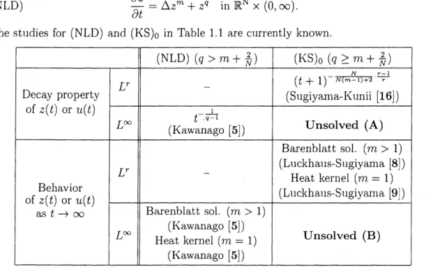
This is analogous to the following nonlinear degenerate heat equation:
(NLD)
$\frac{\partial z}{\partial t}=\triangle z^{m}+z^{q}$ $in\mathbb{R}^{N}\cross(0, \infty)$.
The
studies for (NLD)
and
$(KS)_{0}$
in
Table 1.1
are
currently
known.
Table
1.1.
The known results for (NLD) and
$(KS)_{0}$
with
small initial data.
Therefore
our
aim is to give
an answer
to
the unsolved
part (A)
in Table 1.1.
Before stating
our
result
we define
global weak solutions to
$(KS)_{0}.$
Definition 1.1. Let
$T>0$
.
A
pair
$(u, v)$
of non-negative
functions defined on
$\mathbb{R}^{N}\cross(0, T)$is
called a?veak solution to
$(KS)_{0}$
on
$[0, T$
)
if
(a)
$u\in L^{\infty}(O, T;L^{p}(\mathbb{R}^{N}))(\forall p\in[1, \infty u^{m}\in L^{2}(0, T;H^{1}(\mathbb{R}^{N}))$
,
(b)
$v\in L^{\infty}(O, T;H^{1}(\mathbb{R}^{N}))$
,
(c)
$(u, v)$
satisfies
$(KS)_{0}$
in the
distributional sense,
i.e.,
for
every
$\varphi\in C_{0}^{\infty}(\mathbb{R}^{N}\cross[0,$$T$
$\int_{0}^{T}\int_{\mathbb{R}^{N}}(\nabla u^{m}\cdot\nabla\varphi-u^{q-1}\nablav\cdot\nabla\varphi-u\varphi_{t})dxdt=\int_{\mathbb{R}^{N}}u_{0}(x)\varphi(x, 0)dx,$
$\int_{0}^{T}\int_{\mathbb{R}^{N}}(\nabla v\cdot\nabla\varphi+v\varphi-u\varphi)dxdt=0.$
In
particular,
if
$T>0$
can be taken arbitrarily, then
$(u, v)$
is called
a
global weak solution
We
now
state
our
nlain
result in
this paper.
Theorem
1.1. Let
$N\in \mathbb{N},$$m\geq 1_{f}q\geq 2.$
$Lefm$
and
$q$satisfy
$q>m+ \frac{2}{N}.$
Assume
further
that
$u_{0}$satisfy
(1.1)
and
(1.2)
$\{\begin{array}{ll}\Vert u_{0}\Vert_{L^{N}}\tau^{(qn)}\sim\leq\min\{\delta_{u,\frac{N}{2}(q-m)}, \delta_{u,r_{3)}}\delta_{u,70}\} ?vhen q\geq m+1(N\geq 3) , N=1, 2\Vert u_{0}\Vert_{L^{N}}\tau\leq\min\{\delta_{u,\frac{N}{2})}\delta_{u,7’ 3}, \delta_{u,r0}\} when q<m+1(N\geq 3) ,\end{array}$where
$\delta_{u,r}=\min\{1, \frac{4m}{2^{q-2}rC’}, (\frac{4m(r+q-2)}{2^{q-2}(r+m_{\fbox{Error::0x0000}}-1)^{2}C"})^{\frac{1}{q-m}}\},$
$C’=C’(r, m, q, N)$
,
$C”=C”(r, m, q, N)r_{3}=r_{3}(m, q, N)$
(defined
in subsection
3.2)
and
$r_{0}= \max\{N-m+1, m-3, N(q-m)-m+1\}$
are
positive
$con$
stants. Then
$(KS)_{0}$
has
a
non-negative weak
solution
$(u, v)$
on
$[0, \infty$
)
whzch
satisfies
the
following
decay
property:
(1.3)
$\Vert u(t)\Vert_{L^{\infty}(\mathbb{R}^{N})}\leq Kt^{-\frac{1}{q-1}}=Kt^{-\frac{N}{N(m-1)+2q}}$,
a.a.
$t\in(0, \infty)$
,
(1.4)
$\Vert u(t)\Vert_{L^{\infty}(\mathbb{R}^{N})}\leq K_{\rho}(t+\rho)^{-\frac{N}{N(m-1)+2}}$,
a.a.
$t\in[5\rho, \infty)$
,
where
$q_{*}:= \frac{N}{2}(q-m)$
,
$K=K(\Vert u_{0}\Vert_{Lq*}, C_{r3}, r_{3}, m, q, N)>0$
is
a constant,
$\rho\in(0,1$
]
is
arbitrary
and
$K_{\rho}=K_{\rho}$ $(p, C_{r}r_{3}3,, \Vert u_{0}\Vert_{L^{1}}, |u_{0}\Vert_{Lq*}, \Vert u_{0}\Vert_{L^{r}3)}m, q, N)(arrow\infty as \rhoarrow 0)$
is
a
positive
constant, where
$C_{r}$is the
$consta\uparrow 7t$
given
in
Proposition
2.1.
The
decay
rate in Theorem 1.1
may
be
best
possible,
because of
the
following two
reasons.
First Reason:
As
stated
above,
$(KS)_{0}$
can
be rewritten
$a_{\iota}^{c}$;
the equation (E1)
like
(NLD),
From comparing the
diffusion
term
$\triangle u^{m}$with the
aggregation term
$u^{q}$in (E1),
$(KS)_{0}$
ha
the global
solvability and the solution has
$L^{r}$-decay
property when
$q \geq m+\frac{2}{N}$
and the
initial data is
sufficiently small ([16]). Kawanago [5] showed the
$L^{\infty}$-decay property for
(NLD)
when
$q>m+ \frac{2}{N}$
,
that
is,
if the
initial
data
is
sufficiently small, then (NLD) has
a
global solution which satisfies
$\Vert z(t)\Vert_{L^{\infty}(\mathbb{R}^{N})}\leq M_{0}t^{-\frac{1}{q-1}}=M_{0}t^{-\frac{N}{N(m-1)+2q*}})$
where
$q_{*}= \frac{N}{2}(q-m)$
and
$M_{0}>0$
is
some
constant.
Hence
we
expect
that the
solution
to
$(KS)_{0}$
has
$\Vert u(t)\Vert_{L^{\infty}(\mathbb{R}^{N})}\leq M_{1}t^{-\frac{1}{q-1}}=M_{1}t^{-\frac{N}{N(rn-1)+2q*}},$
where
$1lI_{1}$is
some
constant.
Second Reason:
Sugiyama-Kunii
[16] showed the
$L^{r}$-decay
property of
solutions
to
$(KS)_{0}$
:
(1.5)
$\Vert u(t)\Vert_{L^{r}}\leq C_{r}(1+t)^{-\alpha}, r\in[1, \infty)$
,
where
Giving
an
eye to the decay rate
$\alpha$,
we
have
$\frac{N}{N(m-1)+2}\cdot\frac{r-1}{r}arrow\frac{N}{N(m-1)+2} (rarrow\infty)$
.
Hence
we
expect
that
the solution
to
$(KS)_{0}$
has
$\Vert\prime\int(t)\Vert_{L(\mathbb{R}^{N})}\infty\leq M_{2}t^{-\frac{N}{N(m-1)+2}},$
where
$M_{2}$is
some
constant.
One
of the
difficulties
in
showing the
$L^{\infty}$-decay
estimates
is
that the
coefficient
$C_{r}arrow\infty$
as
$rarrow\infty$
in (1.5)
(see
the definition of
$C_{r}$in Proposition
2.1
below),
and
hence the
$L^{\infty}-$decay
property
is
not
obtained by the limiting proce,ss in
(1.5).
To
evade this
problem
and
obtain the
$L^{\infty}$-decay property
we
establish
the
following
two
kinds of
$L^{\infty}-L^{r}$estimates
without assuming that
the
initial data is small
(see
Section
3):
(I)
$\Vert u(t)\Vert_{L^{\infty}(\mathbb{R}^{N})}^{r-(q_{*}+q-1)}\leq C(r)(\frac{t}{2}\Vert u(\frac{t}{2})\Vert_{L^{r}(\mathbb{R}^{N})}^{r}+(\frac{t}{2})^{1_{-1}}-\frac{r-}{q}L*)$,
(II)
$\Vert u(t)\Vert_{L^{\infty}(\mathbb{R}^{N})}^{r}\leq\tilde{C}(r)(t+\rho)^{-\frac{N}{N(m-1)+2}}(\Vert u(\frac{t}{2}-2e)\Vert_{L^{r}(\mathbb{R}^{N})}^{r}+\Vert u_{0}\Vert_{L^{1}}(t+\rho)^{-\frac{N(r-1)}{N(m-1)+2}}))$where
$q_{*}= \frac{N}{2}(q-m)$
,
$C(r)$
,
and
$\tilde{C}(r)$are
positive constants. We
can
obtain
the
$L^{\infty}-$decay
properties (1.3)
and
(1.4)
by
combining the
$L^{r}$-decay estimate with
(I)
and
(II),
respectively. The condition
$q>m+ \frac{2}{N}$
is necessary
to
show that the coefficient
$\tilde{C}(r)$is
bounded
as
$rarrow\infty$
.
The proofs of
(I)
and
(II)
are
based
on
R.
Suzuki [17]
in
which he
studied the
following
equation:
(E2)
$\frac{\partial z}{\partial t}=\triangle z^{m}+a,$ $\nabla z^{p}+z^{q}$in
$\mathbb{R}^{N}\cross(0, \infty)$,
where
$m\geq 1,$
$p,$
$q>1,$
$a\in \mathbb{R}^{N},$$a\neq$
O. He proved that the solution to
(E2)
has the
following decay property when
$q>m+ \frac{2}{N}$
:
if
the
initial data is
sufficiently
small,
then
$\Vert z(t)\Vert_{L^{\infty}(\mathbb{R}^{N})}\leq M_{3}\min\{t^{-\frac{N}{N(m-1)+2q}}t^{-\frac{N}{N(m-1)+2}\}})$
,
a.a.
$t>0,$
where
$q_{*}= \frac{N}{2}(q-m)$
,
$M_{3}>0$
is
some
constant.
Also
from
this,
we can
expect
that the
solution
to
$(KS)_{0}$
has the
$L^{\infty}$-decay
properties (1.3)
and
(1.4). Moreover,
he showed in
[17] that the solution to
(E2)
behaves like the Barenblatt solution
$(m>1)$
or
the Heat
kernel
$(m=1)$
when
$q>m+ \frac{2}{N}$
and
$p>m+ \frac{1}{N}.$
Finally, we
glance at the unsolved part (B) in
Table 1.1.
From the
known
results
for
the
behavior of solutions ([5], [8], [9] and [17]),
we
conjecture that the solution to
$(KS)_{0}$
ha.s
a
similar
behavior in the
case
where
$q>m+ \frac{2}{N}$
and the initial data is small. This
conjecture will be
discussed in
our
forthcoming paper.
This paper
is organized
as follows.
In
Section
2
we
recall the
$L^{r}$-decay
of solutions
to
$(KS)_{0}$
.
First
we deal
with
the
case
where
$N\geq 2$
in
Section
3,
because the
approximation
is
different between
more
than
one
dimension and
$1D$
.
Section
3
consists of
two
subsections.
Section 3.1
give.
$Q!$the
$L^{\infty}$-bonnd
of solutions to
$(KS)_{0}$
.
Section
3.2
is the main part
of this
paper,
where the
$L^{\infty}$-decay of solutions to
$(KS)_{0}$
is
obtained. Finally
we
consider the
case
2.
$L^{r}$-decay
property
First
we state the result
on
the global
existence
and
$L^{r}$-decay
propertv
of solutions
to
$(KS)_{0}$
.
This
proposition
is stated in [16, Theorem 3].
Proposition
2.1
(global existence of weak solutions to
$(KS)_{0}$
).
Let
$N\in \mathbb{N},$$m\geq 1_{f}$
$q\geq 2$
.
Suppose
that
$m$
and
$q$satisfy
the snper-critical
$CO77$
dition, i.
e.,
$q \geq m+\frac{2}{N}$
Let the initial data
satisfy
(1.1) and
the smallness condition (1.2)
in
Theorem
1.1.
Then
$(KS)_{0}$
has
a
non-negative
global weak
solution
$(u, v)$
which has the
mass
conservation law:
(2.1)
$\Vert u(t)\Vert_{L^{1}(\mathbb{R}^{N})}=\Vert u_{0}\Vert_{L^{1}(\mathbb{R}^{N})}, t\geq 0.$ILforeover,
$t\mapsto\Vert u(t)\Vert_{L^{7}(\mathbb{R}^{N})}(1\leq r<\infty)$
is
a non
increasing
$fu7l$
ctio
7?
$n|ith$
the
$follo?vi_{7}\uparrow g$decay
property:
(2.2)
$\Vert u(t)\Vert_{L^{r}(\mathbb{R}^{N})}\leq C_{r}(1+t)^{-\alpha}, r\in[1, \infty) , t\geq 0,$
where
(2.3)
$\alpha=\frac{N}{N(m-1)+2}.\frac{r-1}{r})$
(2.4)
$C_{r}= \max\{\frac{(r+m-1)^{2}}{r}\cdot\frac{1}{2m(m-1+\frac{2}{N})}(c(N)\Vert u_{0}\Vert_{L^{1}})^{\frac{N}{N(m-1)+2}\frac{r-1}{r}}, \Vert u_{0}\Vert_{L^{r}}\}.$
Remark
2.1. The non-negativity of the solutions is obtained from the standard
argument
and
the comparison principle (see [16]).
Remark
2.2.
In
[16], they
assume
the
smallness
only
$\Vert u_{0}\Vert_{L^{N}}\tau^{(q-n/)}(N\geq 1).$
Howeve
$I^{\cdot}$from
the approximation to the nonlinear term in the first
equation
in
$(KS)_{0}$
,
when
$m+ \frac{2}{N}\leq$$q<m+1(N\geq 3)$ ,
we
should
assume
the smallness of
$\Vert u_{0}\Vert_{L^{\sim}T}N$(see
[4]).
Remark
2.3.
In [16],
it
seems
difficult
to prove the
$L^{\infty}$-bound of the approximate solution
without assuming that
$u_{0}=$
O. Indeed,
they
assume
the
smallness
$\Vert u_{0}\Vert_{L^{\frac{N(q-m)}{l}}}\leq\delta_{u,r}=$$C_{0}r^{-\frac{l}{q-n}}$
to
obtain the
$L^{r}$-estimate.
If
$rarrow\infty$
in this
assumption,
then
it
should be
$\Vert u_{0}\Vert_{L^{\frac{N(q-m)}{l}}}=$
O.
To
overcome
the difficulty
we
give
a
proof
by using Moser’s
iteration
technique
(cf.
R. Suzuki [17,
Section
3.1]),
3. The
case
where
$N\geq 2$
In
this section we establish two kinds of
$L^{\infty}-L^{r}$estimates”’ of solutions
to
$(KS)_{0}$
.
The
first
one
is for the
$L^{\infty}$-bound
(Proposition 3.1)
and
the
second
is
for
$L^{\infty}$-decay property
(Proposition 3.5).
In the end of this section we prove Theorem 1.1
$(N\geq 2)$
.
Now
we
introduce
the
approximate problem:
where
$N\geq 2,$ $m\geq 1,$
$q\geq 2$
and
$\epsilon\in(0,1)$
.
The initial data
$u_{0\epsilon}\in C_{0}^{\infty}(\mathbb{R}^{N})$is
given
as
$u_{0\epsilon}$ $:=(\rho_{\epsilon}*u_{0})\zeta_{\epsilon}$
,
where
$\rho_{\epsilon}$is
a
mollifier
such that
$0\leq\rho_{\epsilon}\in C_{0}^{\infty}(\mathbb{R}^{N})$
,
supp
$\rho_{\epsilon}\subset\overline{B(0,\epsilon)},$ $\int_{\mathbb{R}^{N}}\rho_{\epsilon}(x)dx=1,$and
$\zeta_{\epsilon}$is
a
cut-off
function, i.e.,
$\zeta_{\epsilon}(x)$ $:=\zeta(\epsilon x)$,
where
$\zeta$is
a
fixed function in
$C_{0}^{\infty}(\mathbb{R}^{N})$such
that
$0\leq\zeta\leq 1,$
$\zeta(x)=\{\begin{array}{l}1 (|x|\leq 1) ,0 (|x|\geq 2) .\end{array}$Remark
3.1.
Let
$T>$
O. Let
$u_{\epsilon}$be
a
soh tion to
$(KS)_{\epsilon}$on
$[0, T$
). Then the following
continuity holds:
(3.1)
$\Vert u_{\epsilon}(t)\Vert_{L^{r}(\mathbb{R}^{N})}\in C([0, T])(\forall r\in[1,\infty$Indeed,
reading
the
standard argument
to
$constr\iota lct$
the local
(approximate)
solution
again
(see
[16, Proposition 8, Lemma.s11 and 12],
Amann
[1, Theorem IV.1.5.1]),
we
see that
$u_{\epsilon}\in C([O, TL^{\alpha}(\mathbb{R}^{N}))$for every
$\alpha\in(N, \infty)$
.
This
fact
together
with the
$n$) $ass$
conservation law
(2.1)
implies the continuity
(3.1).
Thib continuity will be used in Lemma
3.3.
Remark
3.2.
If
$u_{0}$satisfies the smallness condition
as
in
Theorem 1.1. then the
approx-imate
solution
$u_{\epsilon}$has
the
same
$L^{r}$
-decay
as
(2.2)
and
$t\mapsto\Vert u_{\epsilon}(t)\Vert_{L^{r}(\mathbb{R}^{N})}$is
a
non
increase
function.
3.1.
$L^{\infty}$-bounds
The next proposition shows the
$L^{\infty}$-bonnd
of the solution
$u$
to
$(KS)_{0}$
.
Indeed, (3.3)
(in
Proposition
3.1)
implies
that
$\Vert u(t)\Vert_{L^{\infty}(\mathbb{R}^{N})}\leq K_{0}a.a.$$t\in(\rho, T)$
for every
$\rho>0.$
Proposition
3.1
(
$L^{\infty}$-estimate of solutions
to
$(KS)_{0}$
).
Let
$N\geq 2,$
$m\geq 1,$
$q\geq 2,$
$\epsilon\in(0,1)$
and
$T>0$
.
Let
$(u, v)$
be
a
weak
solution to
$(KS)_{0}$
on
$[0, T$
).
Assume that
$m$
and
$q$satisfy
(3.2)
$q \geq m+\frac{2}{N}$
and
$u_{0}$satisfies
(1.1)
$a^{!}nd$the
smallness
condition (1.2)
in
Theorem 1.1.
Then
the
follo
$\uparrow$
)
$ing$
estimate
holds:
(3.3)
$\Vert u(t)\Vert_{L^{\infty}(\mathbb{R}^{N})}\leq K_{1}t^{-\frac{N}{N(m-1)+2q*}}$,
a.a.
$t\in(0, T)$
,
where
$q_{*}= \frac{N}{2}(q-m)$
,
$K_{1}=K_{1}(\Vert u_{0}\Vert_{Lq}., C_{r_{1}}, m, q, N)>0$
and
$C_{r}1$is
the
same
constant
as
$ir/$Proposition
2.1.
The proof of this proposition employs the similar method to R. Suzuki [17,
Section
Lemma 3.2.
Let
$N\geq 2,$ $m\geq 1,$
$q\geq 2,$
$\epsilon\in(0,1)_{z}T>0$
and
$0\leq t_{1}<t_{2}\leq T.$
Let
$(u_{\epsilon}, v_{\epsilon})$
be
a
$uniqu\epsilon$solution to
$(KS)_{\epsilon}0\uparrow?[0, T$
). Let
$\psi(t)\in C^{1}([t_{1}, t_{2}])$
with
$0\leq\psi\leq 1,$
$\psi(t_{1})=0,$
$\psi(t_{2})=1$
.
Assume fhut
$m(l7?dq$
satisfy
(3.2).
Then
$foarrow r>(1$
:
(3.4)
$\Vert u_{\epsilon}(t_{2})\Vert_{L^{r-q+1}(\mathbb{R}^{N})}^{r-q+1}+\frac{4m(r-q+1)(r-q)}{(r-q+m)^{2}}\int_{t_{1}}^{t_{2}}\psi(t)\Vert\nabla^{\frac{r}{\epsilon}\Delta\underline{+rn}}u^{2}-(t)\Vert_{L^{2}(\mathbb{R}^{N})}^{2}dt$$+ \epsilon^{m-1}\frac{4m(r-q)}{r-q+1}\int_{t_{1}}^{t_{2}}\psi(t)\Vert\nabla u_{\epsilon}r-\ovalbox{\tt\small REJECT}_{2}+1(t)\Vert_{L^{2}(\mathbb{R}^{N})}^{2}dt$
$\leq\int_{t_{1}}^{t_{2}}\psi’(t)\Vert u_{\epsilon}(t)\Vert_{L^{r-q+1}(R^{N})}^{r-q+1}dt$
$+2^{q-2}(r-q)( \int_{t_{1}}^{t_{2}}\Vert u_{\epsilon}(t)\Vert_{L^{r}(\mathbb{R}^{N})}^{\gamma}dt+\overline{c}m\int_{t_{1}}^{t_{2}}||\tau\iota_{\epsilon}(t)\Vert_{L^{r-q+2}(\mathbb{R}^{V})}^{r-q+2}dt)$
Proof.
Let
$r>2$
.
Multiplying the
first
approximate
equation (1)
by
$u_{\epsilon}^{r-1}$and integrating
it
over
$\mathbb{R}^{N}$,
we obtain
(3.5)
$\frac{1}{r}\frac{d}{dt}\Vert u_{\epsilon}(t)\Vert_{L^{r}(\mathbb{R}^{N})}^{r}$$\leq-\frac{4m(r-1)}{(r+m-1)^{2}}\Vert\nabla u^{\frac{7+n1-1}{\epsilon 2}}(t)\Vert_{L^{2}(\mathbb{R}^{N})}^{2}-\frac{4m(r-1)\epsilon^{m-1}}{r^{2}}\Vert\nablau^{\frac{7}{\epsilon^{2}}}(t)\Vert_{L^{2}(\mathbb{R}^{N})}^{2}$
$+ \int_{\mathbb{R}^{N}}(\prime.\prime J_{\epsilon}\cdot.$
Multiplying
(3.5)
by
$\psi(t)$
and
integrating
it
by
parts
over
$(t_{1}, t_{2})$,
we
see
that
(3.6)
$\Vert u_{\epsilon}(t_{2})\Vert_{L^{r}(\mathbb{R}^{N})}^{r}-\int_{t_{1}}^{t_{2}}\psi’(t)\Vert u_{\epsilon}(t)\Vert_{L^{r}(\mathbb{R}^{N})}^{r}dt$$\leq-\frac{4mr(r-1)}{(r+m-1)^{2}}\int_{t_{1}}^{t_{2}}\psi(t)\Vert\nabla u^{\frac{r+m-1}{\epsilon 2}}(t)\Vert_{L^{2}(\mathbb{R}^{N})}^{2}dt$
$-4m(r-1)\epsilon$
$r m-1 \int_{t_{1}}^{t_{2}}\psi(t)\Vert\nabla u^{\frac{r}{\epsilon^{2}}}(t)\Vert_{L^{2}(\mathbb{R}^{N})}^{2}dt+r\int_{t_{1}}^{t_{2}}\psi(t)I_{2}dt.$
We
denoted by
$I_{2}$the
third term
on
the right-hand side of
(3.5).
We make
an
estimation
of
$I_{2}$.
Letting
$F(s):= \int_{0}^{s}(\tau+\epsilon^{\frac{m}{q-2}})^{q-2}\tau^{r-1}d\tau, \tau\geq 0, s\geq 0, \epsilon\in(0,1)$
and
noting that
we
find
by (2) that
(3.7)
$I_{2}=-(r-1) \int_{\mathbb{R}^{N}}F(u_{\epsilon})\triangle v_{\epsilon}dx$$=-(r-1) \int_{\mathbb{R}^{N}}(v_{\epsilon}-u_{\epsilon})F(u_{\epsilon})dx$
$\leq(r-1)\int_{\mathbb{R}^{N}}u_{\epsilon}F(u_{\epsilon})dx$
$\leq\frac{2^{q-2}(r-1)}{r+q-2}\int_{1R^{N}}u_{\epsilon}^{r+q-1}dx+\frac{2^{q-2}\epsilon^{m}(r-1)}{r}\int_{\mathbb{R}^{N}}u_{\epsilon}^{r+1}dx.$
Hence it
follows
from
(3.6), (3.7)
and
$0\leq\psi\leq 1$
that
(3.8)
$\Vert u_{\epsilon}(t_{2})\Vert_{L^{r}(\mathbb{R}^{N})}^{r}+\frac{4mr(r-1)}{(r+m-1)^{2}}\int_{t_{1}}^{t_{2}}\psi(t)\Vert\nabla u^{\frac{r+m-1}{\mathcal{E}2}}(t)\Vert_{L^{2}(\mathbb{R}^{N})}^{2}dt$$+ \frac{\epsilon^{m-1}4\uparrow?x(r-1)}{r}\int_{t_{1}}^{t\underline{o}}\psi(t)\Vert\nabla u^{\frac{\Gamma}{\epsilon^{2}}}(t)\Vert_{L^{2}(\mathbb{R}^{N})}^{2}dt$
$\leq l_{1}^{t_{2}}\psi’(t)\Vert\uparrow 1_{\epsilon}(t)\Vert_{L^{r}(\mathbb{R}^{N})}^{r}dt$
$+2^{q-2}(r-1) \int_{t_{1}}^{t_{2}}(\frac{r}{r+q-2}\Vert u_{\epsilon}(t)\Vert_{L^{r+q-1}(\mathbb{R}^{N})}^{r+q-1}+\epsilon^{m}\Vert u_{\epsilon}(t)\Vert_{L^{r+1}(\mathbb{R}^{N})}^{r+1})dt.$
Replacing
$r$with
$r-q+1$
in
(3.8),
we
obtain
(3.4)
for
$r>q.$
$\square$Lemma
3.3.
Let
$N\geq 2,$
$m\geq 1,$
$q\geq 2,$
$\epsilon\in(0,1)$
and
$T>$
O.
Let
$(e\iota_{\epsilon}, v_{\epsilon})$be
a
nnique
solution to
$(KS)_{\epsilon}$on
$[0, T$
).
Put
$I=[\tau, \tau+s]a7l(I’=[\tau-\sigma, \tau+s]\iota vith$
$0<\sigma<\tau<\tau+s<T$
.
Put
$q_{*}:= \frac{N}{2}(q-m)$
,
$h$$:=t\in[0,T]\backslash \sigma;up\Vert u_{\epsilon}(t)\Vert_{q}^{q}$
.
and
$r_{*}>q_{*}+q-1$
is
some
constant.
Assume
further
that
$m$
and
$q$satisfy
(3.2)
and
$\delta>0$
satisfies
(3.9)
$\sigma\delta^{q-1}\leq 1.$Then
for
$r\geq r_{*},$
(3.10)
$\mu_{0}(Y_{I,k(r-q+1)+7n-1}+Z_{I,k(r-q+1)})^{\frac{1}{k}}$
$\leq(\frac{4}{\sigma}\delta^{-q+1}+2^{q-1}(r-q))Y_{I’,r}+2^{q-1}\epsilon^{\prime n}(r-q)Z_{I’r-q+2}),$
where
$k:=1+ \frac{2}{N},$
$\mu_{0}=\mu_{0}(h, m, q, N)$
and
$Y_{I,r}:= \int_{I}\int_{\mathbb{R}^{N}}u_{\epsilon}^{r}dxdt+\frac{(s+\sigma)h}{\delta^{q_{*}}}\delta^{r}) Z_{I,r}:=\int_{I}\int_{\mathbb{R}^{N}}u_{\epsilon}^{r}dxdt.$
Proof.
Let
$r>q.$
Fronl
(3.1)
we can
take
$\tilde{t}\in I$such that
Let
$\prime\tilde{\psi}(t):=\frac{t-\tau+\sigma}{\tilde{t}-\tau+\sigma}, t_{1}^{\sim}:=\tau-\sigma, t_{2}^{\sim}:=\tilde{t}$
and note that
$0\leq\tilde{\psi}\leq 1,$ $\tilde{\psi}(t_{1}^{\sim})=0,$ $\tilde{\psi}(t_{2}^{\sim})=1,$ $0 \leq\tilde{\psi}’(t)=\frac{1}{\overline{t}-\tau+\sigma}\leq\frac{1}{\sigma}$and
$[t_{1}^{\sim}, \tilde{t}_{2}]\subset I’$Then
we can
substitute
$\tilde{\psi},$ $t_{1}^{\sim}$and
$\tilde{t}_{2}$into
$\psi,$ $t_{1}$and
$t_{2}$in
(3.4)
and thus, we have
(3.11)
$\max_{t\in I}\int_{\mathbb{R}^{N}}u_{\epsilon}^{r-q+1}(t)dx$
$\leq\frac{1}{\sigma}\int_{I},$$\int_{\mathbb{R}^{N}}u_{\epsilon}^{r-q+1}dxdt+2^{q-2}(r-q)\int_{I’}(\Vert u_{\epsilon}(t)\Vert_{L^{r}(\mathbb{R}^{N})}^{r}+\epsilon^{m}\Vert u_{\epsilon}(t)\Vert_{L^{r-q+2}(\mathbb{R}^{N})}^{r-q+2})dt.$
Next letting
$\hat{\psi}(t):=\{\begin{array}{ll}1, t\in[\tau, \tau+s],-\sigma^{-2}(t-\tau)^{2}+1, t\in[\tau-\sigma, \tau],\end{array}$ $t_{1}^{\wedge}:=\tau-\sigma,$
$t_{2}^{\wedge}:=\tau+s$
and noting that
$0\leq\hat{\psi}\leq 1,$
$\hat{\psi}(t_{1}^{\wedge})=0,$ $\hat{\psi}(t_{2}^{\wedge})=1,$ $0 \leq\hat{\psi}’(t)\leq\frac{2}{\sigma}$and
$I\subset[t_{1}^{\wedge}, t_{2}^{\wedge}]\subset I’$,
we
can
substitute
$\hat{\psi},$ $t_{1}^{\wedge}$and
$t_{2}^{\wedge}$into
$\psi,$ $t_{1}$and
$t_{2}$in
(3.4).
Hence
we
see
that
(3.12)
$v_{0} \int_{I}\Vert\nabla u_{\tilde{\epsilon^{2}}}r+m-(t)\Vert_{L^{2}(\mathbb{R}^{N})}^{2}dt+\epsilon^{m-1}\nu_{1}\int_{I}\Vert\nabla u^{\frac{r}{\epsilon}\Delta_{2}\underline{+1}}-(t)\Vert_{L^{2}(\mathbb{R}^{N})}^{2}dt$
$\leq\frac{2}{\sigma}\int_{I},$
$\int_{\mathbb{R}^{N}}u_{\epsilon}^{r-q+1}dxdt+2^{q-2}(r-q)\int_{I},$
$(\Vert u_{\epsilon}(t)\Vert_{L^{r}(\mathbb{R}^{N})}^{r}+\epsilon^{m}\Vert u_{\epsilon}(t)\Vert_{L^{r-q+2}(\mathbb{R}^{N})}^{r-q+2})dt,$where
$\nu_{0}$ $:= \min\{1, \inf_{r\geq r_{*}}\frac{4m(r-q+1)(r-q)}{(r+m-q)^{2}}\},$ $\nu_{1}$ $:= \min\{1, \inf_{r\geq r_{*}}\frac{4n(r-q)}{r-q+1}\}$and
$r_{*}> \frac{N}{2}(q-m)+q-1$
is
some
constant.
Combining
(3.11)
with (3.12),
we
have
(3.13)
$\max_{t\in I}\int_{\mathbb{R}^{N}}u_{\epsilon}^{r-q+1}(t)dx$$+v_{0} \int_{I}\Vert\nabla u^{\frac{r+m-}{62}}(t)\Vert_{L^{2}(\mathbb{R}^{N})}^{2}dt+\epsilon^{m-1}\nu_{1}\int_{I}\Vert\nabla u^{\frac{r}{\epsilon}\Delta_{2}\underline{+1}}-(t)\Vert_{L^{2}(\mathbb{R}^{N})}^{2}dt$
$\leq\frac{3}{\sigma}\int_{I’}\int_{\mathbb{R}^{N}}u_{6}^{r-q+1}dxdt+2^{q-1}(r-q)(\int_{I}, \Vert u_{\epsilon}(t)\Vert_{L^{r}}^{r}dt+\epsilon^{m}\int_{I}, \Vert u_{\epsilon}(t)\Vert_{L^{r-q+2}}^{r-q+2}dt)$
.
We
estimate the first term
on
the right-hand side of (3.13).
Set
$E_{\delta}(t):= \{x\in \mathbb{R}^{N};u_{\epsilon}(x, t)\geq\delta\})q_{*}:=\frac{N}{2}(q-m) , h:=\backslash s\iota\iota p\Vert u_{\epsilon}(t)\Vert_{Lq*(\mathbb{R}^{N})}^{q_{*}}t\in[0,T|.$
Noting that
$|I’|=s+\sigma$
,
we see
that for
$r \geq\max\{q, r_{*}\}=r_{*}(>q_{*}+q-1)$
,
(3.14)
$\int_{I}, \int_{\mathbb{R}^{N}}u_{\epsilon}^{r-q+1}dxdt=(\int_{I}, \int_{E_{\delta}(t)}+\int_{I}, \int_{\mathbb{R}^{N}\backslash E_{\delta}(t)})u_{\epsilon}^{r-q+1}dxdt$To estimate the left-hand side of
(3.13),
we
use
the
Sobolev
type
inequality
in
[17,
Lemma
2.9]:
(3.15)
$[ \int_{I}\int_{\mathbb{R}^{N}}|f|^{\tilde{\alpha}}dxdt]^{\frac{1}{k}}\leq C_{0}^{\frac{1}{k}}[\max_{t\in I}\int_{\mathbb{R}^{N}}|f|^{a}dx+\int_{I}\int_{\mathbb{R}^{N}}|\nabla f|^{2}dxdt],$where
$\alpha\geq 0,$ $\tilde{\alpha}=2(\frac{\alpha}{N}+1)$,
$k=1+ \frac{2}{N},$
$f\in C(I;L^{\alpha}(\mathbb{R}^{N}))\cap L^{2}(I;H^{1}(\mathbb{R}^{N}))$
and
$C_{0}$is
a
positive
constant depending only
on
$N$
.
Applying
(3.15)
with
$f=u_{\epsilon^{2}}\infty^{r+rn-}$and
$\alpha=\frac{2(r-q+1)}{r-q+7n}$or
$f=u^{\frac{f}{\epsilon}-}\Delta\underline{+1}2$and
$\alpha=2$
,
we
find that for
$r\geq q-1,$
(3.16)
$\{\frac{1}{C_{0}}\int_{I}\int_{\mathbb{R}^{N}}u_{\epsilon}^{k(r-q+1)+m-1}dxdt\}^{\frac{1}{k}}\leq\max_{t\in I}\int_{\mathbb{R}^{N}}u_{\epsilon}^{r-q+1}(t)dx+\int_{I}\Vert\nabla u^{\frac{r+}{\epsilon}R^{m-}}2(t)\Vert_{L^{2}(\mathbb{R}^{N})}^{2}dt,$
(3.17)
$\{\frac{1}{C_{0}}l\int_{\mathbb{R}^{N}}u_{\epsilon}^{k(r-q+1)}dxdt\}^{1}k\leq\max_{t\in l}\int_{\mathbb{R}^{N}}u_{\epsilon}^{r-q+1}(t)dx+l\Vert\nabla u^{\frac{r-}{\epsilon}s_{2}\underline{+1}}(t)\Vert_{L^{2}(\mathbb{R}^{N})}^{2}dt.$Let
$r \geq\max\{r_{*}, q-1\}=r_{*}$
.
Plugging
$(3.16)-(3.17)$
into
(3.14)
to
left-
and right-hand
sides of
(3.13),
respectively, we have
(3.18)
$\frac{\nu_{0}}{2C_{0}^{1/k}}\{\int_{I}\int_{R^{N}}u_{\epsilon}^{k(r-q+1)+m-1}dxdt\}^{\frac{1}{k}}+\epsilon^{m-1}\frac{\nu_{1}}{2C_{0}^{1/k}}\{\int_{I}\int_{\mathbb{R}^{N}}u_{\epsilon}^{k(r-q+1)}dxdt\}^{\frac{1}{k}}$$\leq[\frac{3}{\sigma}\delta^{-q+1}+2^{q-1}(r-q)]\int_{I}, \int_{\mathbb{R}^{N}}u_{\epsilon}^{r}dxdt+\frac{3(s+\sigma)}{\sigma}\delta^{r-q.-q+1}h$
$+2^{q-1}\epsilon^{m}(r-q)l,$
$\int_{R^{N}}u_{\epsilon}^{r-q+2}$(txdt.
Adding
$\frac{s+\sigma}{\sigma}\delta^{r-q_{*}-q+1}h$to the
both sides of
(3.18),
we
obtain
(3.19)
$\frac{\nu_{0}}{2C_{0}^{1/k}}\{\int_{I}\int_{\mathbb{R}^{N}}u_{\epsilon}^{k(r-q+1)+m-1}dxdt\}^{\frac{1}{k}}+\frac{s+\sigma}{\sigma}\delta^{r-q_{*}-q+1}h$ $+ \epsilon^{m-1}\frac{\nu_{1}}{2C_{0}^{1/k}}\{l\int_{\mathbb{R}^{N}}u_{\epsilon}^{k(r-q+1)}dxdt\}^{\frac{1}{k}}$ $\leq[\frac{3}{\sigma}\delta^{-q+1}+2^{q-1}(r-q)]\int_{I}, \int_{\mathbb{R}^{N}}u_{\epsilon}^{r}dxdt+\frac{4}{\sigma}\delta^{-q+1}(s+\sigma)h\delta^{r-q_{*}}$ $+2^{q-1} \epsilon^{m}(r-q)\int_{I’}\int_{\mathbb{R}^{N}}u_{\epsilon}^{r-q+2}dxdt$ $\leq[\frac{4}{\sigma}\delta^{-q+1}+2^{q-1}(r-q)]\{\int_{I}, \int_{\mathbb{R}^{N}}u_{\epsilon}^{r}dxdt+\frac{(s+\sigma)h}{\delta^{q}}\delta^{r}\}$ $+2^{q-1} \epsilon^{m}(r-q)\int_{I’}\int_{\mathbb{R}^{N}}u_{\epsilon}^{r-q+2}dxdt.$Since
$\sigma\delta^{q-1}\leq 1$and
it
follows that
(3.20)
$\frac{(s+\sigma)h}{\sigma}\delta^{r-q_{*}-q+1}=\{\frac{(s+\sigma)h}{\delta^{q_{*}}}\delta^{k(r-q+1)+m-1}\}^{\frac{1}{k}}(\frac{1}{\sigma\delta^{q-1}})^{\frac{1}{k}}(\frac{s+\sigma}{\sigma}h)^{1-\frac{1}{k}}$$\geq h^{1-\frac{1}{k}}\{\frac{(s+\sigma)h}{\delta^{q_{*}}}\delta^{k(r-q+1)+m-1}\}^{\frac{1}{k}}$
Taking (3.20) in the left-hand side of
(3.19)
and using the inequality
$(A+B)^{\frac{1}{k}}\leq A^{\frac{1}{k}}+B^{\frac{1}{k}}$$(A, B>0)$
,
we have
$\mu_{0}\{\int_{I}\int_{\mathbb{R}^{N}}u_{\epsilon}^{k(r-q+1)+m-1}dxdt+\frac{(s+\sigma)h}{\delta^{q_{*}}}\delta^{k(r-q+1)+m-1}$
$+ \epsilon^{m-1}\int_{I}\int_{\mathbb{R}^{N}}u_{\epsilon}^{k(r-q+1)}dxdt\}^{\frac{1}{k}}$
$\leq[\frac{4}{\sigma}\delta^{-q+1}+2^{q-2}(r-q)]$
.
$\{\int_{I},$ $\int_{\mathbb{R}^{N}}u_{\epsilon}^{r}dxdt+\frac{(s+\sigma)h}{\delta^{q_{*}}}\delta^{r}\}$$+2^{q-1} \epsilon^{m}(r-q)\int_{I’}\int_{\mathbb{R}^{N}}u_{\epsilon}^{r-q+2}dxdt,$
where
$\mu_{0}:=\min\{\frac{\nu_{0}}{2C_{0}^{1/k}}, \frac{\nu_{1}}{2C_{0}^{1/k}}, h^{1-\frac{1}{k}}\}$.
Thns
we
obtain
(3.10).
$\square$
Lemma 3.4.
Let
$N\geq 2,$ $m\geq 1,$
$q\geq 2,$
$\epsilon\in(0,1)$
, $T>0$
and
$0<\chi<\tau<\tau+s<T.$
Let
$(u_{\epsilon}, v_{\epsilon})$be
a
unique
solution to
$(KS)_{\epsilon}$on
$[0_{\grave{2}}T$)
Assume thut
$m$
and
$qsatjsf\backslash \uparrow/(3.2)$and
$\delta$satisfies
$\chi\delta^{q-1}\leq 1.$
Then the
following
estimate
holds:
(3.21)
$\Vert u_{\epsilon}\Vert_{L^{\infty}(,sL^{\infty}(\mathbb{R}^{N}))}^{r-(q_{*}+q-1)}1\mathcal{T}\mathcal{T}+)$$\leq[2B(2k)^{\frac{1}{k-1}}]^{\frac{k}{k-1}}\{(1+\epsilon^{m})l_{-\chi}^{\tau+s}\int_{\mathbb{R}^{N}}u_{\epsilon^{1}}^{r}dxdt+(s+\frac{\chi}{2})h\delta^{r-q_{*}}1\},$
where
$k=1+ \frac{2}{N},$
$q_{*}= \frac{N}{2}(q-m)$
,
$r_{1}=r_{1}(m, q, N)\geq 1,$
$h.:=t\in[0_{)}T]s_{\backslash }up\Vert u_{\epsilon}(t)\Vert_{q_{*}}^{q_{*}}a/?d$
$B=B(h, r_{1}, \chi, \delta, m, q, N)>0$
are constants.
Proof.
Let
$q_{*}:= \frac{N}{2}(q-m)$
,
$k:=1+ \frac{2}{N},$
$\lambda_{0}:=q_{*}+q-1,$
$\Lambda_{0}:=\frac{N}{2}+q-1$
and let
$r_{*}>\lambda_{0}$be
some
constant.
First
let
the
sequence
$\{\lambda_{n}\}_{n}\subset \mathbb{R}$be
defined
by
$\{\begin{array}{l}\lambda_{n}=(\lambda_{n-1}-q+1)k+m-1,\lambda_{1}=r_{1}:=\max\{r_{*}, \lambda_{0}, \Lambda_{0}\}.\end{array}$
Thus
Since
$k=1+ \frac{2}{N}>1$
, it follows that
$\lambda_{n+1}>\lambda_{n},$ $r_{1}\leq\lambda_{n}\leq r_{1}k^{n-1}$
and
$\lim_{narrow\infty}\lambda_{n}=\infty.$
Next
define
the sequence
$\{\Lambda_{n}\}_{n}\subset \mathbb{R}a_{u}s$$\{\begin{array}{l}\Lambda_{n}-q+2=(\Lambda_{n-1}-q+1)k,\Lambda_{1}-q+2=r_{1},\end{array}$
and then,
$\Lambda_{n}=\Lambda_{0}+(r_{1}-\Lambda_{0})k^{n-1}$
Since
$k=1+ \frac{2}{N}>1$
,
it
follows that
$\Lambda_{n+1}>\Lambda_{n},$
$r_{1}\leq\Lambda_{n}\leq r_{1}k^{n-1}$
and
$\lim_{narrow\infty}\Lambda_{n}=\infty.$
Let
$I_{n}:=[\tau-2^{-n+1}\chi, \tau+s]$
and
$\delta>0$
such
that
$\chi\delta^{q-1}\leq 1$.
Then
(3.9)
holds for
$\delta$:
$\{(\tau-2^{-n}\chi)-(\tau-2^{-n+1}\chi)\}\delta^{q-1}=(2^{-n}\chi)\delta^{q-1}\leq 1 (n\geq 1)$
and thus,
we can
put
$I=I_{n+1}$
and
$I’=I_{n}$
in (3.10).
Setting
$J_{n}:=l_{n} \int_{\mathbb{R}^{N}}u_{\epsilon}^{\lambda_{n}}dxdt+\frac{(s+2^{-n}\chi)h}{\delta^{q_{*}}}\delta^{\lambda_{n}}+\epsilon^{m}l_{n}\int_{\mathbb{R}^{N}}u_{\epsilon}^{\Lambda_{n}-q+2}dxdt,$
we see
from
(3.10)
that
(3.23)
$\mu_{0}J_{n+1^{\frac{1}{k}}}\leq\{\frac{4}{2^{-n}\chi\delta q-1}+2^{q-1}(\lambda_{n}-q)+2^{q-1}(\Lambda_{n}-q)\}J_{n}.$
Now
we
evaluate the
coefficients
in
(3.23).
Noting
that
$2^{-n}\chi\delta^{q-1}\leq 1,$
$\lambda_{n}\leq r_{1}k^{n-1}$and
$\Lambda_{n}\leq r_{1}k^{n-1}$
,
we
find
that
(3.24)
$\frac{4}{2^{-n}\chi\delta^{q-1}}+2^{q-1}(\lambda_{n}-q)+2^{q-1}(\Lambda_{n}-q)$
$\leq\frac{1}{2^{-n}\chi\delta^{q-1}}\{4+2^{q-1}(\lambda_{n}-q)+2^{q-1}(\Lambda_{n}-q)\}$
$\leq\frac{2^{q-1}}{2^{-n}\chi\delta^{q-1}}(\lambda_{n}+\Lambda_{n})$
$\leq\frac{2^{q}r_{1}}{\chi\delta^{q-1}}2^{n}k^{n-1}$
From
(3.23)
and
(3.24)
it follows that
Therefore
we
obtain
(3.26)
$(J_{n+1})^{\frac{1}{k^{n}}}$$\leq(B\cdot 2^{n}k^{n-1})^{\neg_{k}}1(B\cdot 2^{n-1}k^{n-2})^{\frac{1}{k^{n--}}}\cross\cdots\cross(B\cdot 2)J_{1}$
$=(2B)^{\neg_{k^{n}}-+\frac{1}{k^{n-}}\tau+\cdot\cdot+1}t(2k)^{\neg_{k^{n-+}}\frac{n-2n-}{k}+\cdots+\frac{1}{k}}J_{1}1n-1.$
From
the definition of
$J_{n}$and (3.22)
we
see
that
$\lim_{narrow}\inf_{\infty}(J_{n+1})^{\frac{1}{k^{n}}}\geq\lim_{narrow}\inf_{\infty}(\int_{\tau-2^{-n}\chi}^{\tau+s}\int_{\mathbb{R}^{N}}u_{\epsilon}^{\lambda_{n+1}}dxdt)^{\vec{\lambda_{n+1}}-\lambda_{0}}r\lambda$
$\geq\lim_{narrow}\inf_{\infty}\Vert u_{\epsilon}\Vert_{\tau+s,L^{\backslash _{\iota+1}}’(\mathbb{R}^{N}))}\frac{\backslash _{n+1}}{L^{\backslash _{n+1}}(\mathcal{T}\backslash _{n+1}-\lambda_{0}}r_{1}-\lambda_{0}$
$=\Vert u_{\epsilon}\Vert_{L^{\infty}(\tau,\tau+s,L^{\infty}(\mathbb{R}_{1}^{N}))}^{7_{1}-\lambda_{0}}.$
Hence
it
follows from
(3.26)
that
$\Vert u_{\epsilon}\Vert_{L^{\infty}(\tau,\tau+s;L^{\infty}(\mathbb{R}^{N}))}^{r_{1}-\lambda_{0}}$
$\leq\lim_{narrow}\inf_{\infty}(J_{n+1})^{\urcorner\tau}k1$
$\leq S11\neg 1\frac{1-}{k^{n}\sim}+\cdots+1^{n-1}\neg\frac{n-2}{k^{n--}}+\cdots+\frac{1}{k}$
$=(2B)^{\frac{k}{k-1}}(2k)^{(k-1)} \neg k((1+\epsilon^{n})\int_{\tau-\chi}^{\tau+s}\int_{\mathbb{R}^{N}}u_{\epsilon}^{r_{1}}dxdt+(s+\frac{\chi}{2})h\delta^{r_{1}-q_{*}})$
.
Therefore
we
obtain (3.21).
$\square$Now we prove Proposition
3.1.
From Lemmas
3.2-3.4 we can
obtain
$L^{\infty}-L^{r}$estimate
without assuming that the
initial
data
is
small.
In
the
proof of
Proposition
3.1 we assume
the
smallness condition
of the initial data
to
apply the
$L^{r}$-decay property of
$u_{\epsilon}.$Proof of Proposition
3.1.
Put
$q_{*}:= \frac{N}{2}(q-m)$
,
$k:=1+ \frac{2}{N}$
and let
$r_{*}>q_{*}+q-1$
be
some
constant. Let
$r_{1}$$:= \max\{m+q-2, r_{*}, q_{*}+q-1, \frac{N}{2}+q-1\}$
and
$0<\chi<t<T.$
From Lemma 3.4,
$u_{\epsilon}$satisfies
(3.21).
Moreover,
(3.21)
impJies that
for
a.a.
$0<t<T,$
(3.27)
$\Vert u_{\epsilon}(t)\Vert_{L^{\infty}(\mathbb{R}^{N})}^{r_{1}-(q_{*}+q-1)}$$\leq(2B)^{\frac{k}{k-1}}(2k)^{\frac{k}{(k-1)}z}((1+\epsilon^{m})\int_{t-\chi}^{t}\int_{R^{N}}u_{\epsilon}^{r}1dxds+\frac{\chi}{2}h\delta^{r_{1}-q_{*}})$
,
where
$B= \frac{2^{q}r_{1}}{\mu_{0}\chi\delta q-1}>0,$$h:=t\in[0,T]S11p\Vert u_{\epsilon}(t)\Vert_{Lq*(\mathbb{R}^{N})}^{q_{*}}=1u_{0\epsilon}\Vert_{Lq*}^{q_{*}}$
and
$\mu_{0}=\mu_{0}(m, q_{)}N, h)$
$i$the
same
constant
as
in the proof
of
Lemma
3.3.
Let
$0<t<T.$
$Tal\backslash \prime ing\chi$and
$\delta$such
that
on
$[0, T)$
and using
the
$L^{r}$-decay property
(see
Proposition
2.1
and
Remark
3.2),
we see
that
$\Vert u_{\epsilon}(t)\Vert_{L(\mathbb{R}^{N})}^{r_{1}-(q.+q-1)}\infty\leq C_{1}\{(1+\epsilon^{m})\int_{2}^{t}\int_{\mathbb{R}^{N}}u_{\epsilon}^{r_{1}}dxds+\frac{h}{2}(\frac{t}{2})^{1-\frac{r-q*}{q-1}}\}$
$\leq C_{1}\{(1+\epsilon^{xn})\frac{t}{2}\int_{\mathbb{R}^{N}}u_{\epsilon^{1}}^{r}(\frac{t}{2})dx+\frac{h}{2}(\frac{t}{2})^{1-\frac{r-q}{q-1}}\}$
$\leq C_{1}\{(1+\epsilon^{m})C_{r_{1}}\frac{t}{2}(\frac{t}{2}+1)^{-\frac{N(r_{1}-1)}{N(m-1)+2}}+\frac{h}{2}(\frac{t}{2})^{1_{q}^{r}}-\lrcorner_{\frac{-q*}{-1}}\}$
$\leq C_{1}2^{\frac{r_{1}-q.-q+1}{q-1}}\{(1+\epsilon^{m})C_{r_{1}}+\frac{h}{2}\}t^{-\frac{r-q*-q+1}{q-1}})$
where
$C_{1}=( \frac{2^{q+1}r_{1}}{\mu_{0}})^{\frac{k}{k-1}}(2k)(k\simeq^{k}1)$
and
$C_{r_{1}}$is
the
same
constant
as
in
(2.2).
Thus
we
obtain
(3.28)
$\Vert u_{\epsilon}(t)\Vert_{L\langle \mathbb{R}^{N})}\infty\leq K_{0}(\epsilon)t^{-\frac{1}{q-1}}$$=K_{0}(\epsilon)t^{-\frac{N}{N(m-1)+2q*}}, a.a.
t\in(0, T)$
,
where
$K_{0}( \epsilon)=2^{\frac{1}{q-1}}\{C_{1}(1+\epsilon^{m})C_{r_{1}}+\frac{h}{2}\}^{\frac{1}{r_{1}-(q_{*}+q-1)}}$
It
follows
from
(3.28)
that
for
$a.a.$
$t\in(0, T)$
,
(3.29)
$\Vert u_{\epsilon}(t)\Vert_{L^{\infty}(R^{N})}\leq K_{0}(\epsilon)t^{-\frac{N}{N(n\tau-1)+2q_{*}}}$$\leq K_{0}(1)t^{-\frac{N}{N(m-1)+2q}}.$
This inequality and
$\Vert u_{0\epsilon}\Vert_{L^{r}}\leq\Vert u_{0}\Vert_{L^{f}}(1\leq r\leq\infty)$show that the right-hand side of this
inequality
is independent of
$\epsilon$.
Hence
we
see
that
$\Vert u(t)\Vert_{L\infty(\mathbb{R}^{N})}\leq\lim_{\epsilonarrow}\inf_{0}\Vertu_{\epsilon}(t)\Vert_{L^{\infty}(\mathbb{R}^{N})}$
$\leq$
linl i
$nfK_{0}(\epsilon)t^{-\frac{N}{N(m-1)+2q*}}\epsilonarrow 0$$=K_{1}t^{-\frac{N}{N(n\tau-1)+2q*}}\rangle$
where
$K_{1}$$:=K_{0}(1)>0$
is
a
constant which depends
on
$\Vert u_{0}\Vert_{L^{q*}},$ $C_{r_{1}},$ $r_{1},$$m,$
$q$and
$N.$
Therefore
we
obtain
the desired inequality
(3.3).
$\square$Remark
3.3.
The
estimate
(3.3)
holds for
some
$r\geq r_{1}$
.
In fact,
by recalling the
defini-tions of
$\lambda_{n}$and
$\Lambda_{n_{\backslash }}$,
we see
that
if
$\lambda_{1}=\Lambda_{1}=r$
,
then
(3.3)
holds with
3.2.
$L^{\infty}$-decay
property
In
this subsection
we
prove
the
$L^{\infty}$-decay property
of
solutions to
$(KS)_{0}.$
Proposition
3.5.
(
$L^{\infty}$-decay property) Let
$N\geq 2,$
$m\geq 1,$
$q\geq 2$
and
$\rho\in(0,1$
]. Let
$(u, v)$
be
a global weak solution to
$(KS)_{0}$
on
$[0, \infty$
).
Assume
further
that
$ma7|dq$
satisfy
(3.30)
$q>m+ \frac{2}{N}$
and
$u_{0}$satisfies
(1.1)
$ar/_{ノ}d$the smallness
condition
as
in
Theorem 1.1. Then the solution
$u$
has the following
decay prope
$7^{\tau}ty$:
(3.31)
$\Vert u(t)\Vert_{L^{\infty}(\mathbb{R}^{N})}\leq K_{\rho}(t+\rho)^{-\frac{N}{N(n-1)+2}}$,
a.a.
$t\in[5\rho, \infty)$
,
where
$K_{\rho}=K_{\rho}(\rho, r, C_{r}, \Vert u_{0}\Vert_{L^{1}}, \Vert u_{0}\Vert_{Lq*}, \Vert u_{0}\Vert_{L^{r}}, m, q_{\}}N)$ufith
$q_{*}= \frac{N}{2}(q-m)a77dr\geq r_{3}=$
$r_{3}(m, q, N)$
are
positive
constants and
$C_{r}$is
the
same
constant as
in
$P_{7}$oposition
2.1.
The proof is based
on
[17,
Sections
5-7]. To
this end
we
need
three lemmas.
Lemma
3.6.
Let
$N\geq 2,$
$m\geq 1,$
$q\geq 2,$
$\epsilon\in(0,1)$
,
$\rho\in(0,1$
]
and
$r_{1}$is
the
same
constant
as
in
Section
3.1.
Let
$(u_{\epsilon}, v_{\epsilon})$be a
unique
solution to
$(KS)_{\epsilon}$on
$[0, \infty$
).
Assume
that
$m$
and
$q$satisfy
(3.2)
and
$u_{0}$satisfies
the smallness
$condit\iota on$
as
in Theorem
1,
1.
Then
for
$r\geq r_{1}$
and
$a.a.$
$t\in[2p, \infty$
),
(3.32)
$\Vert u_{\epsilon}(t)\Vert_{L^{\infty}(\mathbb{R}^{N}))}^{r-(q_{*}+q-1)}\leq C_{\rho}’\Vert u_{\epsilon}(t-\rho)\Vert_{L^{r}(\mathbb{R}^{N}}^{r\{1-\Delta_{\frac{-1}{-q*)}(1+\frac{N}{2})\}}}r$where
$q_{*}= \frac{N}{2}(q-m)$
and
$C_{\rho}’=C_{\rho}’(\rho, \epsilon, r, \Vert u_{0\epsilon}\Vert_{L^{r}}, \Vert u_{0\epsilon}\Vert_{Lq*}, m, q, N)>0$is
a
constant.
Proof.
Let
$\rho\in(0,1], r\geq r_{1} (see$
Section
$3.1)$
,
$t\geq 2\rho,$
$q_{*}= \frac{N}{2}(q-m)$
and
$k=1+ \frac{2}{N}.$
Since
$t\mapsto\Vert u_{\epsilon}(t)\Vert_{L^{r}(\mathbb{R}^{N})}$is
a non
increasing
function,
we can
take
$\chi$and
$\delta$
such that
$\chi=\rho, \delta=(\Vert u_{\epsilon}(t-p)\Vert_{\mathbb{R}^{N})}^{\frac{r}{L^{r}(r-q*}})(\Vert u_{0\epsilon}\Vert_{\mathbb{R}^{N})}^{\frac{r}{L^{r}(r-q*}})^{-1}(\leq 1)$
in (3.27)
with
$r_{1}=r$
(see
Remark
3.3). Hence it
follows that for
a.a.
$t\geq 2p,$
$\Vert u_{\epsilon}(t)\Vert_{L^{\infty}(\mathbb{R}^{N})}^{r-(q_{*}+q-1)}$
$\leq C_{\rho}(\Vert u_{\epsilon}(t-\rho)\Vert_{\mathbb{R}^{N})}^{\frac{r}{L^{r}(r-q*}})^{-\frac{(q-1)k}{k-1}}$
$\cross\{(1+\epsilon^{m})\int_{t-\rho}^{t}\Vert u_{\epsilon}(s)\Vert_{L^{r}(\mathbb{R}^{N})}^{r}ds+\frac{\rho h}{2}(\frac{\Vert u_{\epsilon}(t-\rho)||_{L^{r}(\mathbb{R}^{N})}}{||e\iota_{0\epsilon}\Vert_{L^{r}(\mathbb{R}^{N})}})^{r}\}$
$\leq C_{\rho}(\Vert u_{\epsilon}(t-p)\Vert_{\mathbb{R}^{N})}^{\frac{\eta}{L^{r}(r-q*}})^{-\frac{(q-1)k}{k-1}}(\rho(1+\epsilon^{m})+\frac{\rho h}{2}\Vert u_{0\epsilon}\Vert_{L^{r}(\mathbb{R}^{N})}^{-r})\Vert u_{\epsilon}(t-\rho)\Vert_{L’(R^{N})}^{r}$
where
$C_{\rho}=( \frac{2^{q+1}r}{\rho\mu_{0}}\Vert u_{0\epsilon}\Vert^{\frac{r(q-1)}{L^{r}(\mathbb{R}^{N}r-q*}}))^{\frac{k}{k-1}}(2k)^{\frac{k}{(k-1)}}$
and
$\mu_{0}$is
the
same
constant
as
in
the
proof of Lemma
3.3.
Therefore
we obtain
(3.32),
where
$C_{\rho}’=C_{\rho}( \rho(1+\epsilon^{m-1})+\frac{\rho h}{2}\Vert u_{0\epsilon}\Vert_{L^{f}}^{-r})$.
$\square$Lemma
3.7.
Let
$N\geq 2,$
$m\geq 1_{f}q\geq 2,$
$\epsilon\in(0,1)$
,
$\rho\in(0,1] and t\geq 2p.
Let (u_{\epsilon}, ?/_{\zeta})$
be
a
unique
solution
to
$(KS)_{\epsilon}$on
$[0, \infty$
).
Assume
that
$m$
and
$q$satisfy
(3.2).
Put
(3.33)
$G(s) :=(r-1) \int_{0}^{s}(\tau+\epsilon^{\frac{m}{q-2}})^{q-2}d\tau,$
(3.34)
$w_{\epsilon}(x, t) :=u_{\epsilon}e^{-\int_{2\rho}^{t}G(\Vert u_{\epsilon}(s)\Vert_{L^{\infty}(R^{N})})ds}$Then
satisfies
the
following:
(3.35)
$\Vert w_{\epsilon}(t)\Vert_{L^{1}(\mathbb{R}^{N})}\leq\Vert u_{0\epsilon}\Vert_{L^{1}}, t\geq 2\rho,$(3.36)
$\frac{d}{dt}\int_{\mathbb{R}^{N}}w_{\epsilon}^{r-m+1}(t)dx+\mu_{1}\int_{\mathbb{R}^{N}}|\nabla w^{\frac{r}{\epsilon^{2}}}(t)|^{2}dx\leq 0, r>m, t\geq 2\rho)$(3.37)
$t\mapsto\Vert w_{\epsilon}(t)\Vert_{L^{r}(\mathbb{R}^{N})}(1\leq r<\infty)$is
a non-increasing
function
on
$[2\rho, \infty$),
where
$\mu_{1}=\mu_{1}(m)$
is
a
positive
constant.
Proof.
First
we
prove (3.35). From
the
definition
of
$w_{\epsilon}$and
the
mass
conservation law,
we
see
that
for
$t\geq 2\rho,$
$\Vert w_{\epsilon}(t)\Vert_{L^{1}(\mathbb{R}^{N})}\leq\Vert u_{\epsilon}(t)\Vert_{L^{1}(\mathbb{R}^{N})}=\Vert u_{0\epsilon}\Vert_{L^{1}}.$
Thus
we
obtain
(3.35),
Next
we
prove
(3.36). Let
$r>1$
and
$t\geq 2\rho$
.
Differentiating
$w_{\epsilon}$about
$t$,
we see
by
the
first
approximate equation (1)
(see
$(KS)_{\epsilon}$
in
the top of
Section
3)
that
$dw_{\epsilon}$
(3.38)
$–=e^{-\int_{2\rho}^{t}G(\Vert u_{\epsilon}(s)\Vert_{L}\infty)ds}$$dt$
$\cross(\nabla\cdot(\nabla(u_{\epsilon}+\epsilon)^{m}-(u_{\epsilon}+\epsilon^{\frac{m}{q-2}})^{q-2}u_{\epsilon}\nabla v_{\epsilon})-u_{\epsilon}G(\Vert u_{\epsilon}(t)\Vert_{L^{\infty}}))$
.
Multiplying
(3.38)
by
$w_{\epsilon}^{r-1}$and integrating
it
over
$\mathbb{R}^{N}$,
we
have
(3.39)
$\frac{1}{r}\frac{d}{dt}\Vert w_{\epsilon}(t)\Vert_{L^{f}(\mathbb{R}^{N})}^{r}$$=(e^{-r\int_{2\rho}^{t}G(\Vert u_{e}(s)\Vert_{L}\infty)ds}) \cross(\int_{\mathbb{R}^{N}}\nabla\cdot(\nabla(u_{\epsilon}+\epsilon)^{m}-(u_{\epsilon}+\epsilon^{\frac{m}{q-2}})^{q-2}u_{\epsilon}\nabla v_{\epsilon})u_{\epsilon}^{r-1}dx$
$- \int_{\mathbb{R}^{N}}u_{\epsilon}^{r}G(\Vert u_{\epsilon}(t)\Vert_{L\infty})dx)$
By a
similar argument
from
(3.5) to (3.7) in
Lemma
3.2, it
follows
that
(3.40)
$I_{4} \leq-\frac{4m(r-1)}{(r+m-1)^{2}}\Vert\nabla u^{\frac{r+rn-1}{\epsilon 2}}(t)\Vert_{L^{2}(\mathbb{R}^{N})}^{2}-\frac{4m(r-1)\epsilon^{?7l-1}}{r^{2}}\Vert\nabla u^{\frac{r}{\epsilon^{2}}}(t)\Vert_{L^{2}(\mathbb{R}^{N})}^{2}$$+(r-1) \int_{\mathbb{R}^{N}}u_{\epsilon}F(u_{\epsilon})dx,$
where
$F(s):= \int_{0}^{s}(\tau+\epsilon^{\frac{m}{q-2}})^{q-2}\tau^{r-1}d\tau.$
F$ecalling the
definition
of the function
$G$
,
we see that
(3.41)
$(r-1) \int_{\mathbb{R}^{N}}u_{\epsilon}F(u_{\epsilon})dx-I_{5}$$=(r-1) \int_{\mathbb{R}^{N}}\{u_{\epsilon}\int_{0}^{u_{\epsilon}}(\tau+\epsilon^{\frac{m}{q-2}})^{q-2}\tau^{r-1}d\tau-u_{\epsilon}^{r}\int_{0}^{\Vert u_{\epsilon}(t)\Vert_{L}\infty}(\tau+\epsilon^{\frac{m}{q-2}})^{q-2}d\tau\}dx$
$\leq(r-1)\int_{\mathbb{R}^{N}}\{u_{\epsilon}^{r}(\int_{0}^{u_{\epsilon}}-\int_{0}^{\Vert u_{\epsilon}(t)\Vert_{L}\infty})(\tau+\epsilon^{\frac{m}{q-2}})^{q-2}d\tau\}dx$
$\leq 0.$
Hence it follows from
$(3.39)-(3.41)$
that
(3.42)
$\frac{d}{dt}\Vert w_{\epsilon}(t)\Vert_{L^{r}(\mathbb{R}^{N})}^{r}\leq(-e^{-r\int_{2\rho}^{t}G(\Vert u_{\epsilon}(s)\Vert_{L}\infty)ds})\cdot 4mr(r-1)$$\cross(\frac{1}{(r+m-1)^{2}}\Vert\nabla u_{\epsilon^{2}}\mapsto rm-1(t)\Vert_{L^{2}(\mathbb{R}^{N})}^{2}+\frac{\epsilon^{?n-1}}{r^{2}}\Vert\nabla u^{\frac{r}{\epsilon^{2}}}(t)\Vert_{L^{2}(\mathbb{R}^{N})}^{2})$
.
Since
$\Vert\nabla u\Vert_{L^{2}(\mathbb{R}^{N})}^{2}=\frac{r+m-1}{\epsilon 2}(e^{(r+m-1)\int_{2\rho}^{t}G(\Vert u_{\epsilon}\Vert_{L}\infty)ds})\cdot\Vert\nabla w\Vert_{L^{2}(\mathbb{R}^{N})}^{2}\frac{r+m-1}{\epsilon 2}$
by the definition
of
$w_{\epsilon}$,
we see
fronl
(3.42)
that
(3.43)
$\frac{d}{dt}\Vert w_{\epsilon}(t)\Vert_{L^{r}(\mathbb{R}^{N})}^{r}\leq-e^{(m-1)\int_{2\rho}^{t}G(\Vert u_{\epsilon}(s)\Vert_{L}\infty)ds}(r+m-1)^{2}4mr(r-1)\Vert\nabla w\frac{r+\prime n-1}{\epsilon 2}(t)\Vert_{L^{2}(\mathbb{R}^{N})}^{2}.$Replacing
$r$by $r-m+1$
in (3.43)
and
setting
$\mu_{1}:=\inf_{r\geq m}\frac{4m(r-m+1)(r-m)}{r^{2}}$
,
we obtain
(3.36)
for $r>m$
.
Finally
we
prove
(3.37).
From
(3.43)
we see
that for
$r\geq 1,$
$\frac{d}{dt}\Vert w_{\epsilon}(t)\Vert_{L^{r}(\mathbb{R}^{N})}^{r}\leq 0, t\geq 2\rho,$
so
$t\mapsto\Vert w_{\epsilon}(t)\Vert_{L^{r}(\mathbb{R}^{N})}(1\leq r<\infty)$is
a
non-increasing
function
on
$[2p, \infty$
).
$\square$The
next
lemma gives the
$L^{\infty}$-estimate
of
$w_{\epsilon}$.
The lemma similar to
Lemma
3.8
$i_{\backslash }(i$
proved
in
[17,
Section
6],
where they considered the following function
$\overline{w}_{\epsilon}$instead of
$w_{\epsilon}$
:
$\tilde{w}_{\epsilon}(x, t) :=u_{\epsilon}\exp(-\int_{2\rho}^{t}\Vert u_{\epsilon}(s)\Vert_{L^{\infty}(\mathbb{R}^{N})}^{q-1}ds)$
.
next
lemma i
$sp$
roved b
$yu$
sing n
$otthed$
efinition
o
$fw_{\epsilon}Thep$
roof starts w
$ith(3.36)and\iota 1_{\backslash }ses(3.37)$
with
r
$= \frac{2N}{b_{11}tN-1},r=2and(3.35)thep$
roperty o
$fw_{\epsilon}.$.
Lemma
3.8.
Let
$N\geq 2,$
$m\geq 1,$
$q\geq 2,$
$\epsilon\in(0,1)$
and
$\rho\in(0,1].
Let (u_{\epsilon}, v_{\epsilon})$
be
a
unique
solution to
$(KS)_{\epsilon}$on
$[0, \infty$
).
Assume
that
$m$
and
$q$satisfy
(3.2) and
$u_{0}$satisfies
(1.1)
and the
smallness condition
as
in
Theorem
1.1.
Put
$G$
and
$w_{\epsilon}$as
in
(3.33) and (3.34).
Assume
fnrther
that
$\delta’>0$
satisfies
$t^{\frac{1}{2}}\delta^{\prime\frac{1}{N}+\frac{m-1}{2}}\leq 1.$
Then
(3.44)
$\Vert w_{\epsilon}(t)\Vert_{L(\mathbb{R}^{N})}\infty\leq C_{3}((t+\rho)\delta^{\prime m-1})^{-\frac{N}{2}}(\int_{\mathbb{R}^{N}}w_{\epsilon}^{r}(\frac{t}{2}-\frac{\rho}{2})dx+\Vert u_{0\epsilon}\Vert_{L^{1}}\delta^{\prime r-1})$,
$t\geq 5\rho,$
where
$C_{3}=C_{3}(\Vert u_{0\epsilon}\Vert_{L^{1}}, m, q, N)$
is
a
positive
constant.
Proof
of Proposition
3.5.
Let
$\rho\in(0,1], r\geq r_{1} (see$
Section
$3.1)$
and
$t\geq 5\rho$
.
We
use
the
same
notation
as
(3.33)
and
(3.34).
Recalling
the definition of
$w_{\epsilon}$,
we see
that
(3.45)
$\int_{\mathbb{R}^{N}}w_{\epsilon}^{r}(\frac{t}{2}-\frac{\rho}{2})dx\leq\int_{\mathbb{R}^{N}}u_{\epsilon}^{r}(\frac{t}{2}-\frac{\rho}{2})dx,$(3.46)
$\Vert u_{\epsilon}(t)\Vert_{L^{\infty}(\mathbb{R}^{N})}\leq\exp(\int_{2\rho}^{t}G(\Vert u_{\epsilon}(s)\Vert_{L^{\infty}})ds)\Vert w_{\epsilon}(t)\Vert_{L^{\infty}(\mathbb{R}^{N})}.$It
follows from (3.46), (3.44) in Lemma
3.8
and (3.45) that
(3.47)
$\Vert u_{\epsilon}(t)\Vert_{L^{\infty}(\mathbb{R}^{N})}^{r}$$\leq C_{3}e^{r\int_{2\rho}^{t}G(||u_{e}(s)||_{L}\infty)ds}((t+\rho)\delta^{\prime m-1})^{-\frac{N}{2}}(\int_{\mathbb{R}^{N}}u_{\epsilon}^{r}(\frac{t}{2}-\frac{\rho}{2})dx+\Vert u_{0\epsilon}\Vert_{L^{1}}\delta^{\prime r-1})$
.
Take
$\delta’=(t+\rho)^{-\frac{N}{N(m-1)+2}}$
in (3.47). It follows from the
$L^{r}$-decay property of
$u_{\epsilon}$
(see (2.2)
in Proposition
2.1
and
Remark
3.2)
that
$\Vert u_{\epsilon}(t)\Vert_{L^{\infty}(\mathbb{R}^{N})}^{r}\leq C_{3}e^{r\int_{2\rho}^{t}G(\Vert u_{e}(s)||_{L}\infty)ds}$
$\cross(t+\rho)^{-\frac{N}{N(m-1)+2}}(\int_{\mathbb{R}^{N}}u_{\epsilon}^{r}(\frac{t}{2}-\frac{\rho}{2})dx+\Vert u_{0\epsilon}\Vert_{L^{1}}(t+p)^{-\frac{N(r-1)}{N(m-1)+2}})$
$\leq C_{3}C_{r}^{r}e^{r\int_{2\rho}^{t}G(||u_{\epsilon}\langle s)\Vert_{L}\infty)ds}$
$\cross(t+\rho)^{-\frac{N}{N(m-1)+2}}((\frac{t}{2}-\frac{\rho}{2}+1)^{-\frac{N(r-1)}{N(m-1)+2}}+\Vert u_{0\epsilon}\Vert_{L^{1}}(t+\rho)^{-\frac{N(r-1)}{N(m-1)+2}})$
$=C_{4}e^{r\int_{2\rho}^{t}G(\Vert u_{\epsilon}(s)\Vert_{L}\infty)ds}(t+\rho)^{-\frac{Nr}{N(m-1)+2}},$
where
$C_{4}=C_{3}C_{r}^{r}(2^{N(m-1)+2}N(r-1)+\Vert u_{0\epsilon}\Vert_{L^{1}})$
,
$C_{3}$
and
$C_{r}$are
the same constants
as
in Lemma
3.
$S$and Proposition 2.1, respectively.
Hence
we
have
Here
we
estimate
the
function
$G$
.
From
(3.32)
in Lemma
3.6
and the
$L^{T}$-decay
property
(2.2), it follows that a.a.
$t\geq 2\rho,$
(3.49)
$\int_{2\rho}^{t}G(\Vert u_{\epsilon}(s)\Vert_{L^{\infty}(\mathbb{R}^{N})})ds$$=(r-1) \int_{2\rho}^{t}\int_{0}^{\Vert u_{\xi}(s)\Vert\infty}L_{n}(arrow$
$= \frac{r-1}{q-1}\int_{2\rho}^{t}\{(\Vert u_{\epsilon}(s)\Vert_{L^{\infty}(\mathbb{R}^{N})}+\epsilon^{\frac{m}{q-2}})^{q-1\frac{m(q-1)}{q-2}}-\epsilon\}ds$ $\leq\frac{r-1}{q-1}\int_{2\rho}^{t}\{(\prime^{r\{1-A_{\frac{-1}{)^{q*}}(1+\frac{N}{2})\}\frac{1}{-(q*+q-1)}}}r-,.+\epsilon^{\frac{m}{q-2}})^{q-1}-\epsilon^{\frac{1t(q-1)}{q-2}}\}ds$ $\leq\frac{r-1}{q-1}\int_{2\rho}^{t}\{(C_{5}(s-\rho+1)^{-\beta}+\epsilon^{\frac{m}{q-2}})^{q-1}-\epsilon^{\frac{m(q-1)}{q-2}}\}ds,$where
$\beta=\frac{N(r-1)}{N(m-1)+2}\{1-\frac{q-1}{r-q_{*}}(1+\frac{N}{2})\}\frac{1}{r-(q_{*}+q-1)},$
$C_{\rho}’$
is
the
same
constant
as
in
(3.32)
and
$C_{5}=C_{5}(C_{\rho}’, C_{r}, r, m, q, N)$
is a
positive
constant,
Fronl
(3.29) (see the
proof of
Proposition 3.1), (3.48)
and
(3.49)
we see
that
a.a.
$t\geq 1,$
(3.50)
$\Vert\uparrow/(t)\Vert_{L^{\infty}(R^{N})}$ $\leq\lim_{\epsilonarrow}\inf_{0}\Vert u_{\epsilon}(t)\Vert_{L^{\infty}(\mathbb{R}^{N})}$ $\leq\lim_{\epsilonarrow}\inf_{0}\{C^{\frac{1}{4^{r}}}\exp(\int_{2\rho}^{t}G(\Vert u_{\epsilon}(s)\Vert_{L^{\infty}(\mathbb{R}^{N})})d_{\langle}s)(t+\rho)^{-\frac{N}{N(\tau r)-1)+2}}\}$ $\leq\lim_{\epsilonarrow}\inf_{0}[C^{\frac{1}{4r}}\exp(\frac{r-1}{q-1}\int_{2\rho}^{t}\{(C_{5}(s-\rho+1)^{-\beta}+\epsilon^{\frac{rr\iota}{q-2}})^{q-1}-\epsilon^{\frac{rn(q-1)}{q-2}}\}ds)$$\cross(t+\rho)^{-\frac{N}{N(m-1)+2}}]$
$=C_{4}^{\frac{1}{r}} \exp(\int_{2\rho}^{t}C_{6}(s-p+1)^{-\beta(q-1)}ds)(t+\rho)^{-\frac{N}{N(m-1)+2}}$
$\leq C^{\frac{1}{4r}}\exp(\int_{2\rho}^{\infty}C_{6}(s-\rho+1)^{-\beta(q-1)}ds)(t+\rho)^{-\frac{N}{N(m-1)+\underline{o}}},$
where
$C_{6}= \frac{C_{5}(r-1)}{q-1}$.
When
$q>m+ \frac{2}{N}$
,
we have
$- \beta(q-1)=-\frac{N(q-1)}{N(m-1)+2}\{1-\frac{q-1}{r-q_{*}}(1+\frac{N}{2})\}\frac{r-1}{r-(q_{*}+q-1)}$
Hence
there exists
$r_{2}$such that
$-\beta(q-1)<-1$
for
$r\geq r_{2}$
.
It
follows
that
for
$r\geq r_{2},$
(3.51)
$\int_{2\rho}^{\infty}C_{6}(s-\rho+1)^{-\beta(q-1)}ds=\frac{C_{6}(\rho+1)^{-\beta(q-1)+1}}{\beta(q-1)-1}.$
Therefore
we
see
from
(3.50)
and
(3.51)
that
for
$r\geq r_{3}$
$:= \max\{r_{1}, r_{2}\},$
$\Vert u(t)\Vert_{L^{\infty}(\mathbb{R}^{N})}\leq K_{\rho}(t+\rho)^{-\frac{N}{N(m-1)+2}},$
where
$K_{\rho}$ $C_{4}^{\frac{1}{r}} \exp(\frac{C_{6}(\rho+1)^{-\beta(q-1)+1}}{\beta(q-1)-1})$.
This is the required decay property.
$\square$
Proof
of Theorem
1.1
when
$N\geq 2.$
$Fro\ln$
Propositions
3.1
and
3.5
with
$r=r_{3}$
(see
the proof of Proposition
3.5)
we
see
that
$\Vert u(t)\Vert_{L^{\infty}(\mathbb{R}^{N})}\leq\{\begin{array}{ll}Kt^{-\frac{N}{N(m-1)+2q*}}, a.a.t\in(0, \infty) ,K_{\rho}(t+\rho)^{-\frac{N}{N(m-1)+2}}, a.a.t\in(5\rho, \infty) ,\end{array}$
where
$q_{*}= \frac{N}{2}(q-m)$
,
$\rho\in(0,1], K=K(\Vert u_{0}\Vert_{L^{r}3)}C_{r_{3}}, r_{3}, m, q, N)>0$
and
$K_{\rho}=$
$K_{\rho}(\rho, \Vert u_{0}\Vert_{L^{1}}, \Vert u_{0}\Vert_{Lq}., 1u_{0}\Vert_{L^{r}3}, C_{r}3, r_{3}, m, q, N)>0$
are
constants,
where
$C_{r}$is the
same
constant
as
in Proposition 2.1. Thus we obtain
(1.3)
and
(1.4).
$\square$4. The
case
where $N=1$
In
this section
we
consider
the
case
where
$N=1$
. First
we
introduce the approximate
problem when
$N=1.$
$(KS)_{\epsilon,N=1}$
$\{\begin{array}{ll}\frac{\partial u_{\epsilon}}{\partial t}=\frac{\partial^{2}}{\partial x^{2}}(u_{\epsilon}+\epsilon)^{m}-\frac{\partial}{\partial x}(u_{\epsilon}^{q-1}\frac{\partial v_{\epsilon}}{\partial x}) in \mathbb{R}\cross(0, T) , \cdots (1)_{\epsilon,N=1}0=\frac{\partial^{2}v_{\epsilon}}{\partial x^{2}}-v_{\epsilon}+u_{\epsilon} in\mathbb{R}\cross(0, T)) . ..(2)_{\epsilon,N=1}u_{\epsilon}(x, 0)=u_{0\epsilon}(x) , x\in \mathbb{R},\end{array}$where
$m\geq 1,$
$q\geq 2$
and
$\epsilon\in(0,1)$
.
The initial data
$u_{0\epsilon}\in C_{0}^{\infty}(\mathbb{R})$is
given
as
$u_{0\epsilon}$$:=$
$(\rho_{\epsilon}*u_{0})\zeta_{\epsilon)}\cdot\rho_{\epsilon}$
is the mollifier and
$\zeta_{\epsilon}$is
the standard cut function.
Note
that the
nonlinear
term in the first equation of
$(KS)_{\epsilon,N=1}$
is different
from the
approximate nonlinear term in the
ca.se
where
$N\geq 2$
(see
$(KS)_{\epsilon}$in
Section
3).
The
reason
is
that the condition
$q \geq m+\frac{2}{N}$
gives
$q\geq 3$
when
$N=1$
. This condition relates with
$\Vert\nabla u_{\epsilon}(t)\Vert_{L^{\infty}(\mathbb{R}^{N})}$
$(see [16,$
Proposition
$9$Differentiating
$the$
nonlinear term
$\nabla(u^{q-1}\nabla v)$$i’n(KS)_{0}$
about.r formally
to
obtain the estimate of
$\Vert\nabla\uparrow J_{\epsilon}(t)\Vert_{L}\infty(\mathbb{R}^{N})$,
we
see
that
$\frac{\partial}{\partial x_{j}}\nabla(u^{q-1}\nabla v)=(q-1)(q-2)\sum_{i=1}^{N}u^{q-3}\frac{\partial u}{\partial x_{j}}\frac{\partial u}{\partial x_{i}}\frac{\partial v}{\partial x_{i}}$