Some Numerical Results of Rising Bubble Problems (Mathematical Analysis of Viscous Incompressible Fluid)

Some

Numerical

Results of Rising Bubble

Problems

Masahisa Tabata

Department of Mathematics,

Waseda

University

1

Introduction

We consider two-fluid flow problems, where each fluid is governed by the

Navier-Stokes equations and the surface tension proportional to the curvature acts on the

interface. The domain which each fluid occupies is unknown, and the interface

moves with the velocity of the particle on it. While numerical solution of

one-fluid flow problems governed by the Navier-Stokes equations has been successfully

established from the point of stability and convergence, it is not an easy task to

construct numerical schemes solving the two-fluid flow problems. To the best ofour

knowledge there are no numerical schemes whose solutions are proved to converge

to the exact one and there is very little discussion even for the stability of schemes

[1]. Recently we have developed an energy-stable Lagrange-Galerkin finite element

scheme for the two-fluid flow problems [8]. The scheme is anextension of the

energy-stable finite element scheme proposed by us [6, 7] to the Lagrange-Galerkin method.

In this report we present some numerical results of rising bubble problems solved

by it.

2

Two-fluid flow

problems

Let $\Omega$ be

a bounded domain in $R^{2}$ with piecewise smooth boundary $\Gamma$, and $(0, T)$

be a time interval. The domain $\Omega$ is occupied by $m+1$ immiscible incompressible

viscous fluids. Each fluid $k$, whose density and viscosity are

$\rho_{k}$ and $\mu_{k}$, occupies

an unknown domain $\Omega_{k}(t)$ at time $t$. Fluid $k(=1, \cdots, m)$ is surrounded by fluid $0,$

and thesurface tension acts on the interface $\Gamma_{k}(t)$. Let the coefficient of the surface

tension be $\sigma_{k}.$ $\Gamma_{k}(t)$ is expressed as a closed curve,

$\Gamma_{k}(t)=\{\chi_{k}(s, t);s\in[0, 1$

where

$\chi_{k}:[0, 1 ) \cross(0, T)arrow \mathbb{R}^{2}, \chi(1, t)=\chi(0, t) (t\in(O, T))$

is a function to be determined. $\Omega_{k}(t)$, $k=1,$

$\cdots,$$m$, is the interior of $\Gamma_{k}(t)$, and

fluid $0$ occupies

Unknown functions $(u,p)$, velocity and pressure,

$u:\Omega\cross(0, T)arrow \mathbb{R}^{2}, p:\Omega\cross(0, T)arrow \mathbb{R}$

and $\chi_{k}$ satisfy the system ofequations,

$\rho_{k}\{\frac{\partial u}{\partial t}+(u\cdot\nabla)u\}-\nabla[2\mu_{k}D(u)]+\nabla p=\rho_{k}f,$ $x\in\Omega_{k}(t)$, _{$t\in(O, T)$} (1a)

$\nabla\cdot u=0, x\in\Omega_{k}(t) , t\in(O, T)$ (1b)

$[u]=0, [-pn+2\mu D(u)n]=\sigma_{k}\kappa n, x\in\Gamma_{k}(t) , t\in(0, T)$ (1c)

$\frac{\partial\chi_{k}}{\partial t}=u(\chi_{k}, t) , s\in[O, 1 ) , t\in(O, T)(1d)$

$u\cdot n=0,$ $D(u)n\Vert n,$ $x\in\Gamma,$ _{$t\in(O, T)$} (1e) $u=u^{0}, x\in\Omega, t=0$ _(1f)

$\chi_{k}=\chi_{k}^{0}, s\in[0, 1 ) , t=0, (lg)$

where $k=0,$ $\cdots,$$m$ in (1a) and (1b), $k=1,$ $\cdots,$$m$ in (1c), (1d) and $(lg)$, and

$f:\Omega\cross(0, T)arrow \mathbb{R}^{2}, u^{0}:\Omegaarrow \mathbb{R}^{2}, \chi_{k}^{0}:[0, 1)arrow \mathbb{R}^{2}$

are given functions; $f$ is an acceleration, $u^{0}$ is

an initial velocity, $\chi_{k}^{0}$ is a function

showing the initial interface position. means the difference of the values

ap-proached from both sides to the interface, $\kappa$ is the curvature of the interface, and

$n$ is the unit normal. On the boundary of $\Omega$

the slip boundary condition (1e) is imposed.

Lagrange-Galerkin method has nice features for the approximation of material

derivative terms [2, 3, 4, 5]. Since the basic idea is to approximate the particle

movement along characteristic curves, the method is robust for high Reyonolds

number problems. Recently developed energy-stable Lagrange-Galerkin scheme for

two-fluid flow problems is an extension of the energy-stable finite element scheme

[6, 7] to the Lagrange-Galerkin method. It has the following advanteges. For the

details refer to [8].

$\bullet$ It is stable in the sense of energy if an

integral of the square of approximate

curvature of the interface remains bounded.

$\bullet$ Since the resultant

matrix is symmetric, we can use efficient solvers for

sym-metric system of linear equations, e.g., MINRES.

$\bullet$ Sinceweusetheinterface-trackingmethod, we candistributemuch

more

nodes

on the interface than the level-set method.

$\bullet$ When it is applied to incompressible viscous one-fluid flow problems,

the

sta-bility and convergence is assured.

$\bullet$ Since the main computation part is similar to that of the

Stokes problem, the

computation is light.

We apply this scheme to rising bubble problems to analyse the effect of the

3

Numerical results

3.1

Example 1

Let $m=1$ and set

$\Omega=(0,1)\cross(0,4)$,

$\Omega_{1}=\{(x_{1}, x_{2});(x_{1}-a)^{2}+(x_{2}-2a)^{2}<a^{2}\}, a=^{\underline{1}}$

5’

$\rho_{0}=100,$ $\mu_{0}=0.05$, 0.5, 5.0, $\rho_{1}=0.1,$ $\mu_{1}=1.0,$

$f=(0, -1)^{T}, \sigma_{1}=2.0.$

When the viscosity $\mu_{0}$ of fluid $0$ varies, we observe the change ofthe bubble

move-ment depending on $\mu_{0}$. The mesh for the computation is shown in the left of Fig. 1.

We set the time increment $\triangle t=1/16$

.

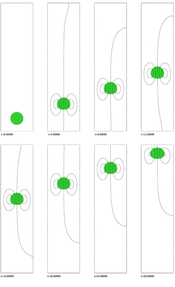
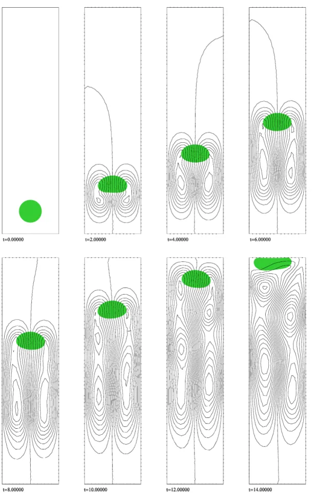
the interfaces and streamlines when $\mu_{0}=5.0$,0.5,0.05. When $\mu_{0}=5.0$, that is, the

viscosity is large, the rising speed of the bubble is slow and any wakes are hardly

visible after the bubble. When $\mu_{0}=0.5$, that is, the viscosity decreases, the rising

speed of the bubble increases and there appear large wakes after the bubble. When

$\mu_{0}=0.05$, that is, the viscosity is small, the rising speed of the bubble becomes high

and there appears oscillation when the bubble rises up. The wake has a pattern

similar to the K\’arm\’an vortex in the flow past a circular cylinder.

3.2

Example 2

Let $m=1$ and set

$\Omega=(0,1)\cross(0,2)$,

$\Omega_{1}=\{(x_{1}, x_{2});(x_{1}-a)^{2}+(x_{2}-2a)^{2}<a^{2}\}, a=\underline{1}$

5’

$\rho_{0}=100, \mu_{0}=0.05, \rho_{1}=0.1, \mu_{1}=1.0,$

$f=(0, -1)^{T},$ $\sigma_{1}=2.0$, 4.O.

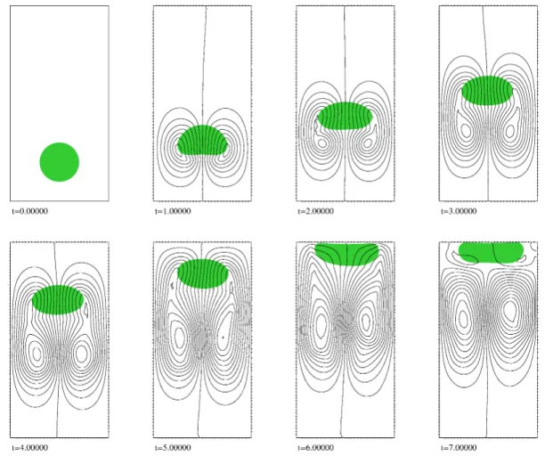
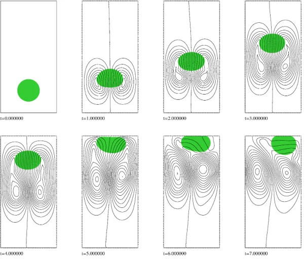
When the coefficient of surface tension$\sigma_{1}$ varies, we observe thechange of the bubble

shape depending on $\sigma_{1}$

.

1. We set the time increment $\triangle t=1/32$. Figs. 5 and 6 show the time histories of

the interfaces and streamlines when $\sigma_{1}=2.0$ and 4.0. When $\sigma_{1}$ increase from 2.0

to 4.0, the shapes ofthe bubbles become more round and the change of the bubble

shapes in the time history becomes smaller.

4

Concluding

remarks

We have analyzed numerically the effect of the viscosity and the coefficient of

sur-face tension on the behavior ofrising bubbles. Our scheme is an interface-tracking

Figure 1: Meshes for Example l(left) and Example2(right).

$N_{e}$ is 2,174 and the number of degrees of freedom $DOF(u,p)$ of the velocity and

pressure is 10,186. In Example 2 $N_{e}$ is 4,564 and $DOF(u,p)$ is 21,021. $DOF(u,p)$

is equal to the size of the system of linear equations solved at each time step. The

$P2/P1/P0$ _finite element spaces are used for the approximation of$u,p$ and $\rho.$

References

[1] E. B\"ansch, Finite element discretization of the Navier-Stokes equations with a

free capillary surface, $Numei_{\mathcal{S}}che$ Mathematik, Vol. 88, No. 2, pp. 203-235, 2001.

[2] O. Pironneau. Finite Element Methods

_for

&

Chich-ester, 1989.

[3] H. Notsu and M. Tabata. Error estimates of a pressure-stabilized chaacteristics

finite element scheme for the Oseen equations. Journal

_of

_Scientific

$t=0.00000$ $t=4.00\mathfrak{o}\mathfrak{o}\mathfrak{o}$ $t=8.\mathfrak{o}\mathfrak{o}000$ _$t=12.00000$

$)$

$t=16.0\mathfrak{o}\mathfrak{o}00$ $t=20.0000\mathfrak{o}$ $t=24.00000$ $t=2S.$_OOOOO

[4] H. Notsu and M. Tabata. Error estimates of a stabilized Lagrange-Galerkin

scheme for the Navier-Stokes equations, to appear.

[5] H. Rui and M. Tabata. A mass-conservative characteristic finite element scheme

for convection-diffusion problems. Journal

_{of Scientific}

416-432, 2010.

[6] M. Tabata. Finite element schemes based on energy-stable approximation for

two-fluid flow problems with surface tension. Hokkaido Mathematical Journal,

Vol. 36, No. 4, pp. 875-890, 2007.

[7] M. Tabata. Numerical simulation of fluid movement in an hourglass by an

energy-stable finite element scheme. In M. N. Hafez, K. Oshima, and D. Kwak,

editors, ComputationalFluidDynamics Review2010, pp. 29-50. WorldScientific,

Singapore, 2010.

[8] M. Tabata. Energy-stable Lagrange-Galerkin schemes for two-fluid flow

prob-lems, to appear.

Department of Mathematics

Waseda University

Tokyo, 169-8555

JAPAN

$E$-mail address: [email protected]

$\rangle$

$\mathscr{B}$

$t=0.00000$ $t=2.00\mathfrak{o}\mathfrak{o}\mathfrak{o}$ $t=4.\mathfrak{o}\mathfrak{o}0\mathfrak{o}\mathfrak{o}$ _$t=6.00000$

$t=8.00000$ $t=10.00000$ $t=12.00000$ $t=14.00000$

$|=0.00000$ $t=2.\mathfrak{o}\mathfrak{o}0\mathfrak{o}\mathfrak{o}$ $|=4.00\mathfrak{o}\mathfrak{o}\mathfrak{o}$ $t=6.\mathfrak{o}0\mathfrak{o}\mathfrak{o}0$

$t=8.\mathfrak{o}\mathfrak{o}0\mathfrak{o}0$ $t=10.0\mathfrak{o}\mathfrak{o}\mathfrak{o}\mathfrak{o}$ $t=12.0\mathfrak{o}\mathfrak{o}\mathfrak{o}\mathfrak{o}$ $|=14.\mathfrak{o}0\mathfrak{o}\mathfrak{o}0$

$t=0$ooooo $t=1(K)(K)($ $t=20\infty 00$ $t=300000$

$t=4$00000 $t=5(KK)00$ $t=6$₀₀₀₀₀ $t=7000\alpha)$

$b)$ $d$

$t=0.(KK)(KK)$ $t=1$(KKKK)O $t=2$000000 $t=3$(KKK)(X)

$t=4(($KKKK) $t=5$(KKK)00 $t=6$(KKKK)0 $t=7$(KKK)00