A Model for Occurrence of Turbulence in Circular Pipe Flows : Experimental Definition of the Problem (Generation-Sustenance Mechanism and Statistical Law of Turbulence)

AModel

for

Occurrence

of

Turbulence

in Circular Pipe

Flows:

Experimental

Definition of the Problem

会津大・理工 神田英貞 (Hidesada Kanda)

Univ. of Aizu, Dept. of Computer Sci. and Engr.

Abstract

Aconceptual model was constructed for the problem of determining the condi-tions under which the transition from laminar to turbulent flow in circular pipes and between parallel plates occurs, so that it becomes possible to calculate the critical Reynolds number (Re). Up until now this problem has been investigated by stability theory with disturbances. However, the minimum critical Reynolds number (Rc(min)) has not yet been obtained theoretically. Accordingly, the author .took up the problem directly ffom many previous experimental investigations and

found that (i) plotsof the transition length versus the Reynolds number (Re) show

that the transition occurs in the entrance region under the conditions of natural

disturbances, _and (ii) plots of ${\rm Re}$ versus the ratio $(\gamma)$ of bellmouth diameter (BD)

to the pipe diameter (D) show that with larger shapes ofbellmouths, laminar flow will persist to higher ${\rm Res}$

.

The problem is thus defined clearly as: Entrance shape

dete rmines the critical Reynolds number.

1Kanda’s

Transition

Model

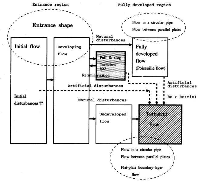
Alayout of the procedure for the modeling and simulation of this problem to determine

${\rm Re}$ is illustrated in Fig. 1on the 7th page. Hence,

we

shall focus

on

the transition length,

which is the distance between the pipe inlet and the point where transition from laminar to turbulent flow occurs, and

on

the shape of bellmouths fitted at the pipe inlet. The

objectives of this study

are

to derive and verify the concepts of the model from previous

experimental investigations, especially (1) - (3), and (6) below.

(1) Transition

occurs

in the entrance region under the conditions of natural disturbances

(Kanda and Oshima, 1987).

(2) Entrance shape determines ${\rm Re}$ apparently: with larger shapes ofbellmouths, laminar

flow will persist up to higher ${\rm Res}$ (Kanda, $1999\mathrm{a}$).

(3) Rc(min) ofapproximately 2000 is obtained in the

case

of astraight circular pipe, i.e.,

when

no

bellmouth is fitted

on

the pipe inlet (Kanda, $1999\mathrm{a}$ and $1999\mathrm{b}$).

(4) The model holds for flows in circularpipes and between parallel plates, i.e., for internal flows (Kanda, 2001).

(5) For external flow such

as

boundary-layer flow past aflat plate, transition occurs

necessarily further downstream since its steady state does not exist (Kanda, $2000\mathrm{a}$).

(6) Disturbances

are

not considered in the current version of the model (Kanda, $2000\mathrm{b}$).

数理解析研究所講究録 1285 巻 2002 年 106-113

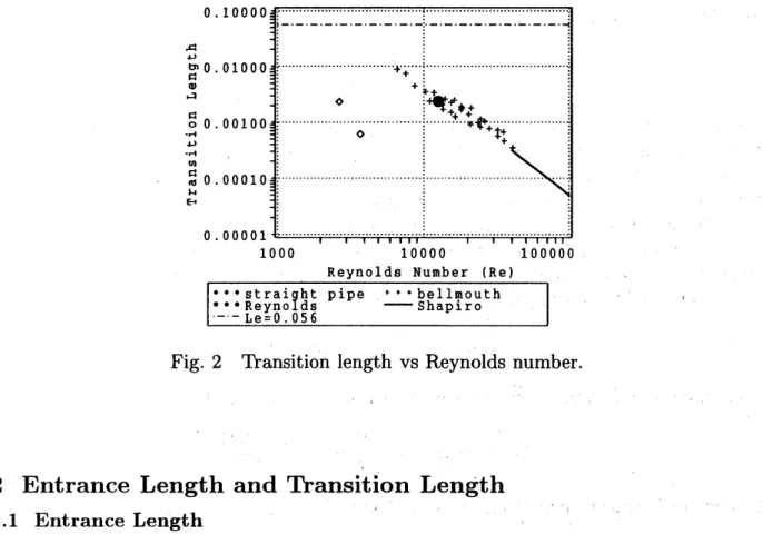
Fig. 2Transition length

vs

Reynolds number.

2Entrance Length

and

Transition

Length

2.1 Entrance Length

The transition length should be compared to the entrance length. The uniform velocity

profile at the pipe inlet is gradually transformed further downstream into the parabolic,

Poiseuille-type distribution by the action of viscous forces on the wall. The entrance

length (Ze) is the distance between the pipe inlet and the point where the velocity profile

giow$\iota\backslash \cdot$ into the fully developed, parabolic distribution. The downstream region after the point $7^{\rho},$. is called the fully developed region. The dimensionless entrance length (Le) is

usually expressed as

Le $\equiv\frac{Ze}{D\cross Re}$

Shah and London (1978) defined Le

as

the point where the developing centerline velocity

equals 99% of the Poiseuille value $u_{\max}$, and recommended the following correlation for

Le:

Le $= \frac{0.6}{Re(1+0.035Re)}$ +0.056 (1)

From Eq. (1), Le varies for ${\rm Res}$ below about 100; however, it approachesaconstant value

of 0.056 for ${\rm Res}$ above 600 (see the constant line of Le $=0.056$ in Fig. 2).

2.2 Transition Length

When the transition length (Zt) is compared to the entrance length, the

same

dimension-less unit is desirable and the dimensionless transition length (Lt) is thus defined by

$Lt$ $\equiv\frac{Zt}{D\cross Re}$

For Reynolds’ color-dye experiments (1883), Lt

can

be estimated

as

$Lt$ $\approx\frac{30}{12,600}=0.00238$ (2)

Figure 2shows the experimental data of Lt, where the diamond and plus symbols show

the transition _{length for flow in the straight pipe and through the bellmouth entrance,}

respectively (Kanda and Oshima, 1987). Theblackdot is the result of Reynolds’ color-dye

experiments. _{The straight line is drawn according to the result of Shapiro and Smith’s}

experiments (1948), in which ${\rm Re}$ (based

on

the pipe diameter) ranged

from 39,000 to

590,000. Shapiro and Smith found that transition from alaminar to turbulent boundary

layer

occurs

at aReynolds number (Rz, based

on

the distance (z) from the pipe inlet) of about 500,000, which compares _{well with the corresponding figure for aflat plate, i.e.,}

$Rz \equiv\frac{zu_{0}}{\nu}=500,000$ (3)

From Shapiro and Smith’s experimental results, Lt is expressed

as

$Lt$ _{$= \frac{z}{DRe}=\frac{Rz}{(Re)^{2}}=\frac{500,000}{(Re)^{2}}$ (4)}

If Reynolds’ critical value of 12,600 is applied to Eq. (4), Lt becomes

$Lt= \frac{500,000}{12,600*12,600}=0.00315$ ₍₅₎

Although this value of 0.00315 is to

some

_{extent larger than the value of 0.00238, which}

is calculated using Eq.(2), they

are

of the

same

order ofmagnitude.

The majorconclusion for Lt is that under the conditions of ordinary disturbances, the

.transition

should necessarily take place in the entrance region.

$Lt<<$ Le $(\approx$ 0.056$)$ (6)

3Effects

of

Bellmouth

3.1 Previous Assumptions

on

the Bellmouth

Bellmouths

are

designed to have the following effects

on

the entrance flow:

(1) The entrance to the pipe is well rounded, and the fluid enters smoothly from

areser-voir, having

an

almost uniform velocity

over

the pipe inlet

cross

section.

(2) The entrance region begins at the pipe inlet, and not at the bellmouth inlet.

Ac-cordingly, the entrance length is measured

as

the distance between the pipe inlet and the

point at which the velocity profile grows into afully developed parabolic distribution.

(3) The fluidwill alwayshave

some

residualdisturbances carried along with it. Bellmouths

are

used to minimize disturbances prior to flow entering the pipe.

The author however showed that abellmouth creates aflow field similar to that in

Fig. 3Reynolds’ bellmouth (a). Fig. 4Reynolds’ bellmouth (b).

the entrance region (Kanda, 1998): (i) At the bellmouth outlet, the axial velocity is not uniform but develops aprofile somewhat similar to Poiseuille’s parabolic profile, because

large vorticities occur on the bellmouth wall and then spread from the wall into the

fluid; (ii) Since radial pressure distributions exist, Prandtl’s boundary-layer assumption

for pressure does not hold for the entire bellmouth region. 3.2 Bellmouth Shapes and Critical ${\rm Re}$

We shall focus on the shape of bellmouths, especially on the ratio (7) of bellmouth

diameter to pipe diameter and consider what determines $\mathrm{R}\mathrm{e}$. Figures 3and 4show the

Reynolds’ bellmouths in his color-dye experiments. Results of previous experimental

investigations are listed in Table 1. Figure 5is drawn by selecting entrances whose sizes

are well describ $\mathrm{e}\mathrm{d}$: Nos. 1.10 and 16 in Table 1.

The major conclusions for the relation between ${\rm Re}$ and

$\gamma$ are as follows:

(1) ${\rm Re}$ takes the minimum value Rc(min) when

$\gamma$ approaches alimit of one.

$Rc( \min)=$ $\lim_{\gammaarrow 1}Rc\approx$ 2000 (7)

(2) With the same shape as the Reynolds’ bellmouth, ${\rm Re}$ increases proportionally to

$\gamma$

as

Eq. (8).

$Rc \approx\gamma\cdot Rc(\min)$ (8)

For Kanda and Oshima’s value of$5790<\mathrm{R}\mathrm{c}<6690$, ${\rm Re}$ is estimated using _$\gamma=2.9$,

$Rc\approx 2.9\cross 2000$ $\approx 5,800$

For Reynolds’ critical value of 12,600, ${\rm Re}$ is estimated using _{$\gamma=5.78$},

$Rc\approx 5.78\cross 2000$ $\approx 11,560$

For Shapiro’ critical value of $\mathrm{R}\mathrm{c}<113,800$, ${\rm Re}$ is estimated using _{$\gamma=46.2$},

$Rc\approx 46.2\cross 2000$ $\approx 92,400$

The values calculated above

are

fairly close to their experimental values of ${\rm Re}$

$\alpha w_{\mathrm{i}}$ $oe\omega$

Ut.U

$\tilde{\mathrm{U}\mathrm{t}6}$ $.r\prec$ $.\mathrm{d}$ $. \downarrow \mathrm{J}\frac{\mathrm{d}}{\mathrm{U}}$ $\omega$ $. \frac{\mathrm{d}}{\mathrm{o}}$

Fig. 5Rc vs bellmouth shape $\gamma$

.

Fig. 6 ${\rm Re}$ using Reynolds’ apparatus.

4General

Questions

on

Disturbances

The present situation of the study of the transition in pipe flows is not obvious. The

obscure comprehension may be caused partly by Ekman’s experimental results and partly

by Van Dyke’s introduction of acurrent critical value when using the same Reynolds’

color-dye experimental apparatus. The three different critical Reynolds numbers (Res)

were

presented (see Fig. 6):

(i) Reynolds: $11.800<\mathrm{R}\mathrm{c}<14,100$; (ii) Ekman: $12,900<\mathrm{R}\mathrm{c}$. $<51,200$;

$l\mathrm{i}\mathrm{i}_{1}).\backslash ^{\gamma}\mathrm{a}\mathrm{n}$ Dyke: _{$\mathrm{R}\mathrm{c}<13,000$}

.

It is thought that this difference is due to different disturbances in flows. It, however,

may be natural to obtainnearly the

same

results anywhere and anytime if fluid dynamics

is scientifically based, such

as

Rc(min) ofapproximately 2000.

(1) Ekman’s

case

(Ekman, 1910)

Kanda(2000b) noted that in thefirst section of Ekman’s paper, the word wax wasused five times: “After the trumpet mouth had been rigidly attached to the glass tube, both were

covered inside, in the neighborhood of thejoint, by alayer of soft

wax. .

.

.

The trumpet

mouth

was now

fastened

more

rigidly, and the

wax

joint

was

improved. Apreliminary

experiment (No. 4).

. .

gave amuch higher value of the critical Reynolds number $\ldots$.”

Apparently, the application of

wax

made ${\rm Re}$ increase to 51,000. Then, concerning the

wax, is it true that the

wax

coated

on

the joint could directly decrease disturbances? The author considers asfollows using the normal wall strength (Kanda, $1999\mathrm{b}$), which

is the radial component of the curl of vorticity multiplied by $(2/{\rm Re})$ (see Eq.(9)).

normal wall strength $\equiv$ $\frac{2}{Re}[\nabla\cross\omega]_{f}|_{r=R}=$ $- \frac{2}{Re}\frac{\partial(v}{\partial z}|_{r=R}$ $>0$ (9)

where $\omega$ is the vorticity, $\mathrm{r}$ the radial coordinate, and $\mathrm{R}$ the pipe radius

(1) the viscosity of the wax is higher than that ofwater; (ii) ${\rm Re}$ is inversely proportional

to viscosity; (iii) the normal wall strength varies inversely to $\mathrm{R}\mathrm{e}$;(iv) the higher viscosity

of thewax caused the normal wall strength to be much higher than in the

case

of without

wax (Reynolds’ experiments) and thus ${\rm Re}$ increased, and; (v) in the

case

of without

wax

(No. 2and 3), Ekman’s results

are

nearly equal to that of Reynolds: ${\rm Re}$ $=\mathrm{a}\mathrm{p}\mathrm{p}\mathrm{r}\mathrm{o}\mathrm{x}\mathrm{i}\mathrm{m}\mathrm{a}\mathrm{t}\mathrm{e}\mathrm{l}\mathrm{y}$

$13,000$.

(2) Van Dyke’s

case

Van Dyke (1982) states: “.. . the original apparatus has survived at the University of

Manchester. Using it acentury later, N. H. Johannesen and C. Lowe have taken this

sequence of photographs. .

. .

Modern traffic in the streets of Manchester made ${\rm Re}$ lower

than the value 13,000 found by Reynolds.”

Professor J. D. Jackson of the University of Manchester kindly allowed the author

to take photographs of the original apparatus on May 25, 1994 (see Figs. 3and 4).

_Of

the original apparatus, the bellmouths (trumpet mouths) have been safely kept in the glass

case there. The bellmouth currently used at the University of Manchester differs from the

original ones, so that ${\rm Re}$ observed by Johannesen and Lowe differed from the results of

Reynolds’ experiments.

Conclusions

The following conclusions are derived under the condition of an ordinary disturbance or

anatural one in flow.

(1) The transition from laminar to turbulent flow occurs in the entrance region since the dimensionless transition length (Lt) is less than 0.01 for most experiments.

(2) It is the shape of pipe entrances that determines the critical Reynolds number (Re).

With larger $\backslash ;$] $.\cdot\cdot \mathfrak{v}\mathrm{e}\mathrm{s}$ ofbellmouths, laminar flow

$\mathrm{w}\mathrm{i}1^{1}1$persist upto higher Reynoldsnumbers.

(3) The $\mathrm{m}\mathrm{i}1:\mathrm{i}\mathrm{r}_{-1}\mathrm{u}\mathrm{m}$ critical Reynolds number (Rc(min)) ofapproximately 2000 is obtained

in the following two cases:

(i) The first

case

is from the Reynolds’ pressure experiments; i.e., when fluid is initially

admitted in ahigh state ofdisturbance, asthe fluidproceeds along the pipe, the turbulent flow settles down to astable condition. Above Rc(min), the turbulent flow never settles

down to astable condition.

(ii) The second is from the experimental data plotted in Fig. 5; in the case of astraight

circular pipe only, i.e., when no bellmouth is fitted on the pipe inlet.

(4) Although there is apparently amarked difference in phenomena between (3-i) and

$(3- \mathrm{i}\mathrm{i})\backslash$

’the

theory of the occurrence of transition and the theory of the settlement of turbulence should be the same (Kanda, $2000\mathrm{a}$).

References

[1] Ekman, V. W., 1910, Arch. Mat. Astron. Fys., bd. 6, no. 12, 1.

[2] Goldstein, S., 1965, Modern Developments in Fluid Dynamics, Vol. 1, 319.

[3] Kanda, H., 2001, ASME FED-Vol. 256, 189.

[4] Kanda, H., 2000a, ASME FED-Vol. 253, 611.

[5] Kanda, H., 2000b, ASME FED-Vol. 253, 619

[6] Kanda, H., 1999a, ASME FED-Vol. 250, 189.

[7] Kanda, H., 1999b, ASME FED-Vol. 250, 197.

[8] Kanda, H., and Oshima, K., 1987, ISAS Report SP No. 5, ISAS Tokyo.

[9] Leite, R. J., 1959, J. ofFluid Mech., Vol. 5, 81.

[10] Reynolds, O., 1883, Trans. Roy. Soc. Lond., Vol. 174, 935.

[11] Reshotko, E., 1958, Jet Propulsion Lab. Progress Report No. 20-364.

[12] Rivas, M. A., and Shapiro, A.H., 1956, Trans. ASME, April, 489.

[13] Senecal, V. E., and Rothfus, R. R., 1953, Chem. Engineering Progress, Vol. 49, 533.

[14] Shah, R. K., and London, A. L., 1978, Laminar Flow Forced Convection in Ducts,

Academic Press, 98.

[15] Shapiro, A.H., and Smith, R.D., 1948, NACA TN No. 1785.

[16] Stanton, T. E., and Pannel, J. R., 1914, Trans. Roy. Soc, Vol. A214, 194.

[17] Van Dyke, M., 1982, An Album of Fluid Motion, Parabolic Press, Stanford, 61.

Entrance region Fully developed region

Fig. 1Modeling and simulation

113

Table 1Critical Reynolds numbers and entrance shapes

[note] Length is in units of cm